Bazykin’s predator-prey ecosystem¶

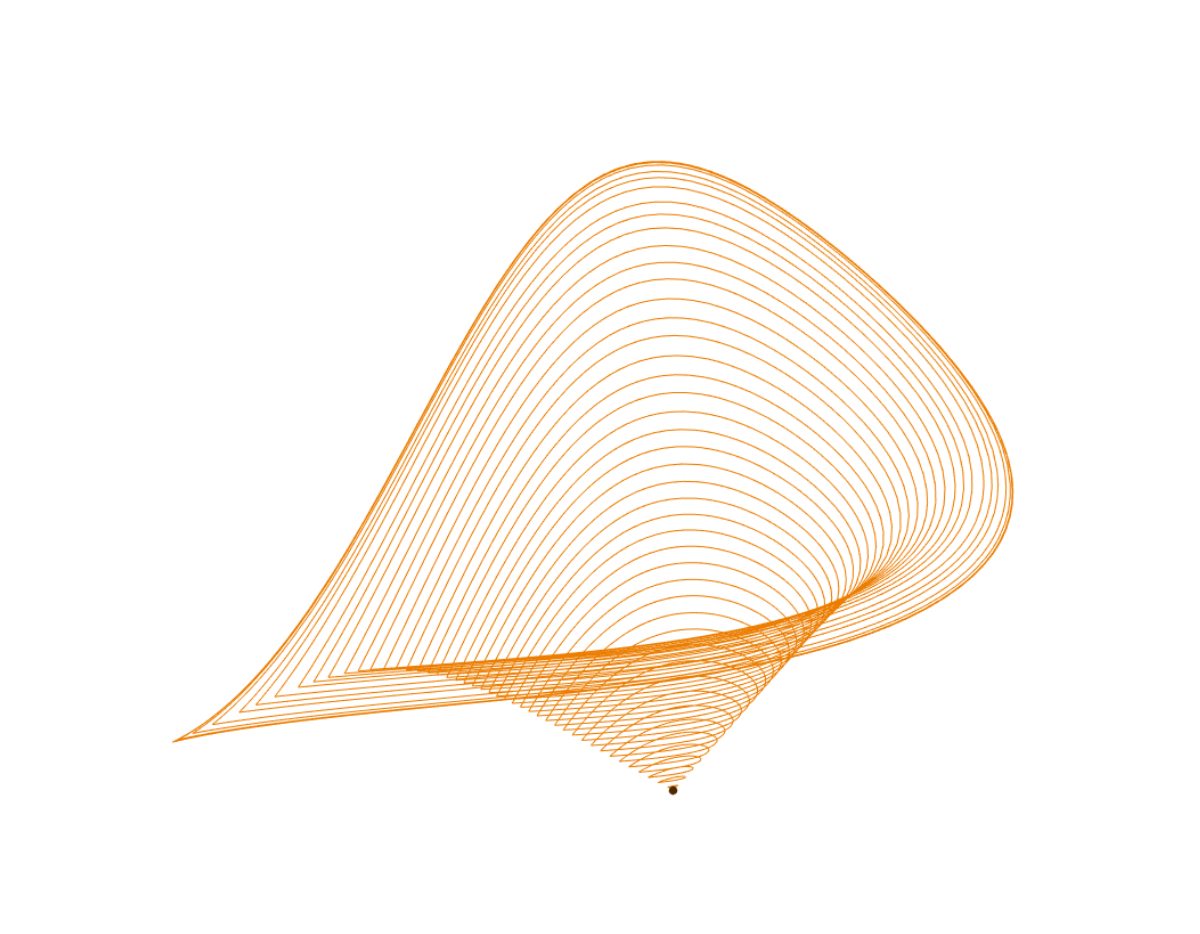
This notebook demonstrates initialization of homoclinic orbits emanating form a generic codimension two Bogdanov-Takens bifurcation point in the following predator-prey ecosystem

\[\begin{split} \begin{cases} \begin{aligned} \dot x_1 &= x_1 - \frac{x_1 x_2}{1+\alpha x_1} - \epsilon x_1^2, \\ \dot x_2 &= -\gamma x_2 + \frac{x_1 x_2}{1+\alpha x_1} - \delta x_2^2. \\ \end{aligned} \end{cases} \end{split}\]

The variables \(x_{1}\) and \(x_{2}\) are (scaled) population numbers of prey and predator, respectively, while \(\alpha, \gamma, \varepsilon\), and \(\delta\) are nonnegative parameters describing the behavior of isolated populations and their interaction, see [Baz85, Kuz04]

Overview¶

In this demo we will

Define an analytically derived Bogdanov-Takens point.
Start continuation of the homoclinic branch emanating from the Bogdanov-Takens point in two parameters \((d,h)\) using the new homoclinic smooth orbital predictor from [Kuz21].
Compare the predicted and computed homoclinic bifurcation curve emanating from the Bogdanov-Takens point in parameters space.
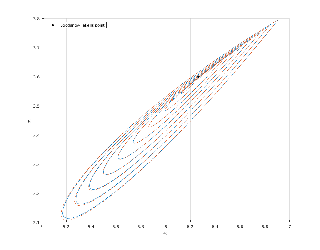
Compare a range of predictors for the homoclinic solutions emanating from the Bogdanov-Takens point with the corrected homoclinic solutions curve in phase-space.
Create a convergence plot of the different homoclinic approximations derived in [Kuz21].

Load MatCont¶

Before we can start using MatCont we need to add the main directory of MatCont, as well as various subdirectories of MatCont, to the MATLAB search path. This is done in the code below. The variable matcont_home should point to the main directory of MatCont.

clear all
matcontpath = '../';
addpath(matcontpath)
addpath([matcontpath, 'Systems'])
addpath([matcontpath, 'Equilibrium'])
addpath([matcontpath, 'LimitPoint'])
addpath([matcontpath, 'LimitPointCycle'])
addpath([matcontpath, 'Hopf'])
addpath([matcontpath, 'Homoclinic'])
addpath([matcontpath, 'LimitCycle'])
addpath([matcontpath, 'Continuer'])
addpath([matcontpath, 'MultilinearForms'])
addpath([matcontpath, 'Utilities'])
set(groot, 'defaultTextInterpreter', 'LaTeX');

Set the odefile¶

Next we set the variable odefile to the system file previously generated by the notebook Generate system files for the Bazykin’s predator-prey system.

odefile=@Bazykin;

Define Bogdanov-Takens point manually¶

It is easy to analytically derive a Bogdanov-Takens point at

\[(x_1, x_2) \approx (6.265765528962353, 3.601553936836365),\]

with parameter values \((\alpha, \delta) \approx (0.4536243277781295, 0.1751275929502174)\).

bt.x = [6.265765528962353; 3.601553936836365];
bt.par = [0.4536243277781295; 0.1751275929502174];

To refer to the parameters throughout the script we create a cell array of strings containing the parameter names. This is then converted into a struct. This allows us to refer to the parameters as ind.parametername, similar as done in DDE-BifTool.

parnames = {'alpha', 'delta'};
cind = [parnames;num2cell(1:length(parnames))];
ind  = struct(cind{:});
ap = [ind.alpha ind.delta]; % continuation parameters

Continue homoclinic curve emanating from Bogdanov-Takens point¶

To continue the homoclinic curve emanating from the Bogdanov-Takens point we use the functions BT_Hom_set_options and init_BT_Hom to obtain an initial approximation to the homoclinic solution (hom_x) as well as a tangent vector to the discretized homoclinic solution (hom_v) as described in Initial prediction of homoclinic orbit near Bogdanov-Takens point 1.

opt = contset;
opt.Singularities = 0;
opt.MaxNumPoints = 300;
opt.MaxStepsize = 1;
options = BT_Hom_set_options();
[hom_x, hom_v] = init_BT_Hom(odefile, bt,  ap, options);
homoclinic_br = cont(@homoclinic, hom_x, hom_v, opt);

Center manifold coefficients' accuracy: 2.664535e-15
BT normal form coefficients:
a=3.945309e-02,	 b=-5.253878e-02
The initial perturbation parameter epsilon:  1.000000e-01
The initial amplitude: 0.857576
The initial half-return time T: 55.2395
The initial distance eps0: 0.00153522
The initial distance eps1: 0.000472271
first point found
tangent vector to first point found

elapsed time  = 11.4 secs
npoints curve = 300

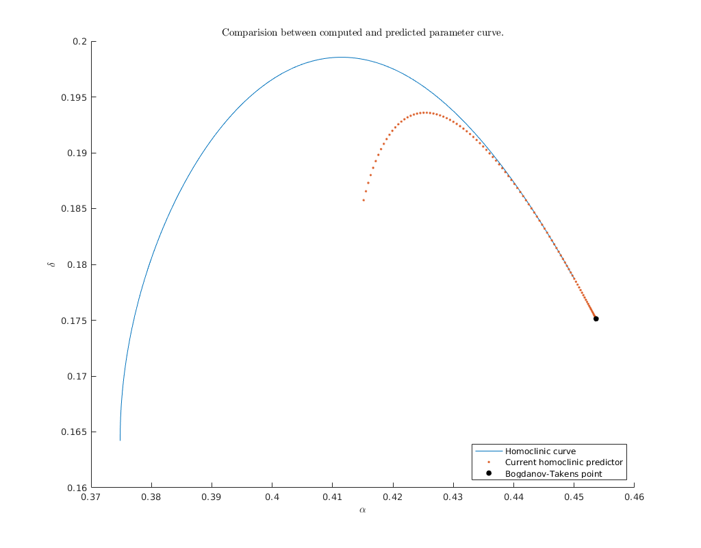
Compare predicted with computed parameters¶

Now that we have obtained a curve of homoclinic orbits (homoclinic_br) we compare the computed curve in parameter space with the predicted curve we construct below. To do so, we use the function BT_nmfm_orbital to obtain the parameter-dependent normal form coefficients and the coefficients between the parameters of the system and the parameters on the center manifold, see [Kuz21].

%plot --width 1024 --height 800
hold on
global homds
% plot computed parameter curve
plot(homoclinic_br(homds.PeriodIdx+1,:), ...
     homoclinic_br(homds.PeriodIdx+2,:));
% Bogdanov-Takens parameter-dependent normal form coefficients
bt = BT_nmfm_orbital(odefile, bt, ap, BToptions);
a   = bt.nmfm.a;
b   = bt.nmfm.b;
K10 = bt.nmfm.K10;
K01 = bt.nmfm.K01;
K02 = bt.nmfm.K02;
K11 = bt.nmfm.K11;
K03 = bt.nmfm.K03;
% construct predictor as in the paper
eps = linspace(0, 0.4);
beta1 = -4*a^3/b^4*eps.^4;
tau0  = 10/7;
tau2  = 288/2401;
beta2 = a/b*(tau0 + tau2*eps.^2).*eps.^2;
alpha = K10.*beta1 + K01.*beta2 + 1/2*K02.*beta2.^2 ...
    + K11.*beta1.*beta2 + 1/6*K03.*beta2.^3;
alpha = bt.par(ap) + alpha;
% plot currect predictor
plot(alpha(1,:), alpha(2,:), '.')
% plot Bogdanov-Takens point
plot(bt.par(ind.alpha), bt.par(ind.delta), '.k', 'MarkerSize', 20)
% set axis labels and legend
xlabel('$\alpha$')
ylabel('$\delta$')
legend({'Homoclinic curve', 'Current homoclinic predictor', ...
    'Bogdanov-Takens point'}, 'Location', 'SouthEast')
%axis([1.1334    1.1658    0.6305    0.7339])
title('Comparision between computed and predicted parameter curve.')

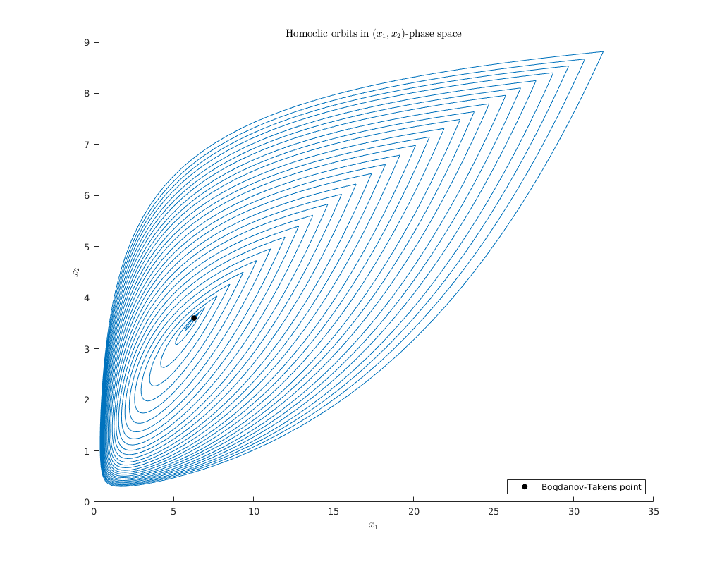
Bifurcation diagram in phase-space \((x_1,x_2)\)¶

To obtain an impression of the homoclinic solutions we plot the computed homoclinic orbits in \((x,y)\) phase-space.

hold on
plot(homoclinic_br(homds.coords(1:homds.nphase:end), 1:10:end), ...
     homoclinic_br(homds.coords(2:homds.nphase:end), 1:10:end), ...
     'Color', [0 0.4470 0.7410], 'HandleVisibility', 'Off')
xlabel('$x_1$')
ylabel('$x_2$')
plot(bt.x(1), bt.x(2), '.k' ,'MarkerSize', 20)
legend('Bogdanov-Takens point', 'Location', 'SouthEast')
title('Homoclic orbits in $(x_1,x_2)$-phase space')

Predictors of orbits for various epsilons¶

Below we compute for a large range of amplitudes the predicted and corrected homoclinic solutions and compare them in phase space. We see that even with an amplitude of 2 the predicted homoclinic orbit is still very close.

options = BT_Hom_set_options();
options.messages = false;
options.correct = false;
options.TTolerance = 1.0e-05;

amplitudes = linspace(1.0e-03, 2,10);
XPredicted = zeros(330,length(amplitudes));
XCorrected = zeros(330,length(amplitudes));
for j=1:length(amplitudes)
  options.amplitude = amplitudes(j);
  [x_pred, v0] = init_BT_Hom(odefile, bt, ap, options);
  XPredicted(:,j) = x_pred;
  try
    XCorrected(:,j) = newtcorr(x_pred, v0);
  catch
    warning('Didn''t convergence to homoclinic solution')
  end
end

hold on
cm = lines;
plot(XPredicted(homds.coords(1:homds.nphase:end),1:10), ...
     XPredicted(homds.coords(2:homds.nphase:end),1:10), ...
      'color', cm(1,:), 'HandleVisibility', 'Off')
plot(XCorrected(homds.coords(1:homds.nphase:end),1:10), ...
     XCorrected(homds.coords(2:homds.nphase:end),1:10), ...
      '--', 'color', cm(2,:), 'HandleVisibility', 'Off')
plot(bt.x(1), bt.x(2), '.k', 'MarkerSize', 16)
xlabel('$x_1$')
ylabel('$x_2$')
legend('Bogdanov-Takens point', 'Location', 'NorthWest')
grid on

Convergence plot¶

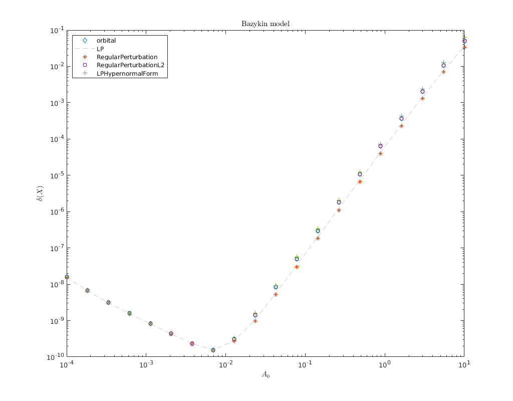
We finish this notebook with a log-log convergence plot comparing the different third order homoclinic approximation methods derived in [Kuz21] to approximate the homoclinic solutions near the first Bogdanov-Takens point. On the abscissa is the amplitude \(A_0\) and on the ordinate the relative error \(\delta\) between the constructed solution (x_pred) to the defining system for the homoclinic orbit and the Newton corrected solution (x_corrected).

BToptions = BT_Hom_set_options();
BToptions.TTolerance = 1e-05;
BToptions.messages = false;
BToptions.correct = false;

amplitudes = logspace(-4, 1, 20);
methodList = {'orbital', 'LP', 'RegularPerturbation', ...
    'RegularPerturbationL2', 'LPHypernormalForm'};
relativeErrors = {};
for i=1:length(methodList)
    BToptions.method = methodList{i};
    relativeErrors{i} = zeros(size(amplitudes));
    for j=1:length(amplitudes)
    BToptions.amplitude = amplitudes(j);
    [x_pred, v0] = init_BT_Hom(odefile, bt, ap, BToptions);
    try
        x_corrected = newtcorr(x_pred, v0);
        relativeErrors{i}(j) = norm(x_corrected-x_pred)/norm(x_corrected);
    catch
        warning('Did not converge.')
        continue
    end
  end
end

cm = lines();
loglog(amplitudes, relativeErrors{1}(:), 'd', ...
       amplitudes, relativeErrors{2}(:), '--', ...
       amplitudes, relativeErrors{3}(:), '*', ...
       amplitudes, relativeErrors{4}(:), 's', ...
       amplitudes, relativeErrors{5}(:), '+')
legend(methodList, 'Location', 'NorthWest')
title('Bazykin model')
xlabel('$A_0$')
ylabel('$\delta(X)$')
ax = gca;
ax.ColorOrder = [cm(1,:); [0.8 0.8 0.8]; cm(2,:); cm(4,:); cm(5,:)];

Interplay between normal forms and center manifold reduction for homoclinic predictors near Bogdanov-Takens bifurcation