Bogdanov-Takens normal form
The universal unfolding for the Bogdanov-Takens normal form is given by
Overview
In this demo we will
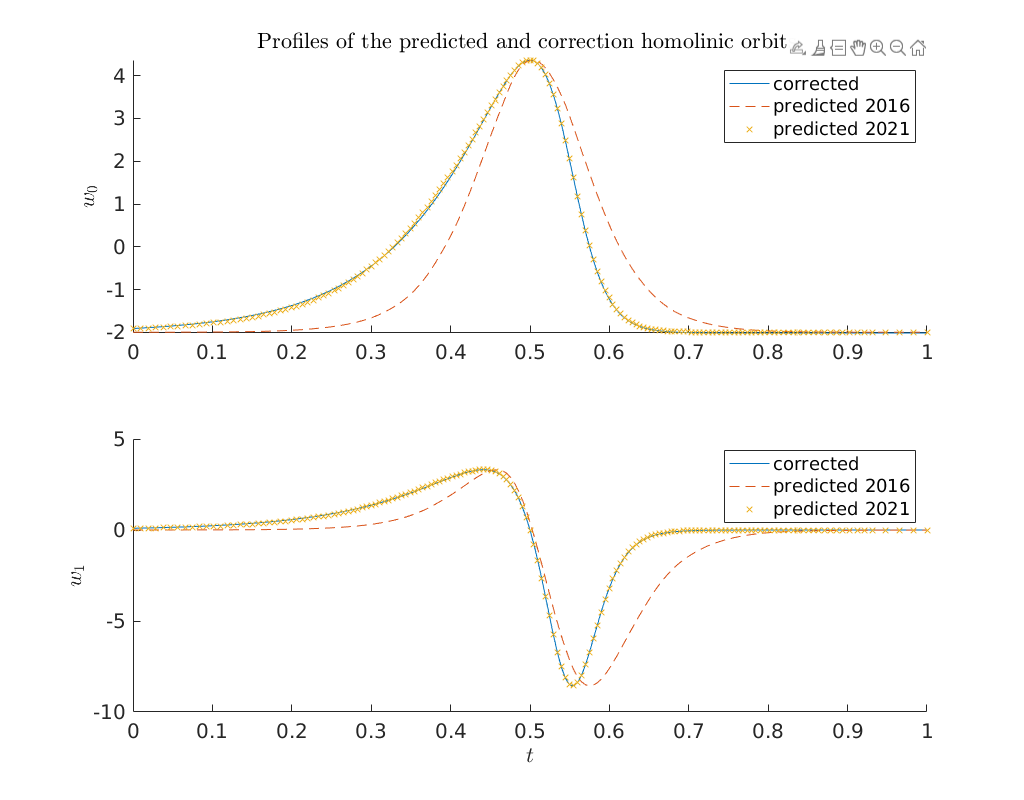
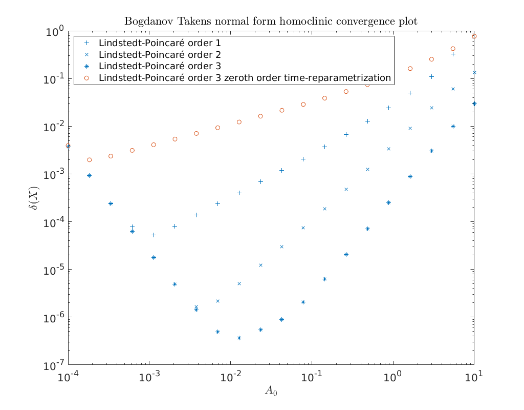
Compare the profiles of the predicted homoclinic solutions emanating from the Bogdanov-Takens point with the corrected homoclinic solutions curve in phase-space. We will do this using the asymptotics derived in [Kuz21] and the asymptotics as provided in [AHGKM16]. We will focus on the difference in using the higher order approximation of the non-linear time transformation.
Create a convergence plot of the different approximation derived in [Kuz21]. And compare them with the approximation derived in [AHGKM16].
This demo will not show how to continue the homoclinic curve emanating from the codimension two Bogdanov-Takens point. For this we refer to one of the other demos.
Load MatCont
Before we can start using MatCont we need to add the main directory of
MatCont, as well as various subdirectories of MatCont, to the MATLAB
search path. This is done in the code below. The variable matcont_home
should point to the main directory of MatCont.
clear all
matcontpath = '../';
addpath(matcontpath)
addpath([matcontpath, 'Systems'])
addpath([matcontpath, 'Equilibrium'])
addpath([matcontpath, 'LimitPoint'])
addpath([matcontpath, 'LimitPointCycle'])
addpath([matcontpath, 'Hopf'])
addpath([matcontpath, 'Homoclinic'])
addpath([matcontpath, 'LimitCycle'])
addpath([matcontpath, 'Continuer'])
addpath([matcontpath, 'MultilinearForms'])
addpath([matcontpath, 'Utilities'])
set(groot, 'defaultTextInterpreter', 'LaTeX');
set(0,'defaultAxesFontSize',15)
Set the odefile
Next we set the variable odefile to the system file previously generated by
the notebook Generate system files for predator-prey system with constant rate harvesting.
odefile=@BogdanovTakensNormalForm;
Define Bogdanov-Takens point
w0 = 0;
w1 = 0;
beta1 = 0;
beta2 = 0;
bt.x = [w0; w1];
bt.par = [beta1; beta2];
To refer to the parameters throughout the script we create a cell array of
strings containing the parameter names. This is then converted into a
struct. This allows us to refer to the parameters as ind.parametername,
similar as done in DDE-BifTool.
parnames = {'beta1', 'beta2'};
cind = [parnames;num2cell(1:length(parnames))];
ind  = struct(cind{:});
Lindstedt-Poincaré with and without higher order time approximation
Here we will show that it is essential to use the higher order approximation of the non-linear time transformation as derived in [Kuz21]. This was not taken into account in [AHGKM16].
%plot --width 1024 --height 800
ap = [ind.beta1, ind.beta2];
BToptions = BT_Hom_set_options();
BToptions.method = 'LP';
BToptions.HigherOrderTimeReparametrization = 0;
BToptions.correct = 0;
BToptions.amplitude = 6;
BToptions.TTolerance = 1.0e-03;
hom2016pred = init_BT_Hom(odefile, bt,  ap, BToptions);
BToptions.HigherOrderTimeReparametrization = 1;
[hom2021pred, hom_v_pred] = init_BT_Hom(odefile, bt,  ap, BToptions);
homcorrected = newtcorr(hom2021pred, hom_v_pred);
global homds
[hom2016predOrbit, saddle2016pred] = bt_rearr(hom2016pred);
[hom2021predOrbit, saddle2021pred] = bt_rearr(hom2021pred);
[homcorrectedOrbit, saddlecorrected] = bt_rearr(homcorrected);
subplot(2,1,1); hold on;
title('Profiles of the predicted and correction homolinic orbits.')
plot(homds.finemsh, homcorrectedOrbit(1:2:end),'-')
plot(homds.finemsh, hom2016predOrbit(1:2:end),'--')
plot(homds.finemsh, hom2021predOrbit(1:2:end),'x')
legend({'corrected', 'predicted 2016', 'predicted 2021'})
ylabel('$w_0$')
subplot(2,1,2); hold on;
plot(homds.finemsh, homcorrectedOrbit(2:2:end),'-')
plot(homds.finemsh, hom2016predOrbit(2:2:end),'--')
plot(homds.finemsh, hom2021predOrbit(2:2:end),'x')
legend({'corrected', 'predicted 2016', 'predicted 2021'})
ylabel('$w_1$')
xlabel('$t$')
BT normal form coefficients:
a=-1,	 b=1
T: 5.04286
The initial perturbation parameter:  1
The initial distance eps0: 0.00144308
The initial distance eps1: 0.00485318
BT normal form coefficients:
a=-1,	 b=1
T: 5.04286
The initial perturbation parameter:  1
The initial distance eps0: 0.112165
The initial distance eps1: 4.58758e-08
Compare predictor and corrected solution in \((w_0, w_1)\) phase-space
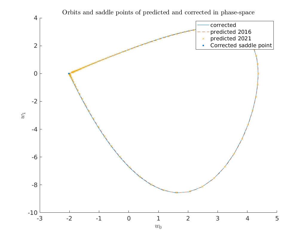
The plot below shows that both predicted homoclinic orbits are in excellent agreement in \((w_0, w_1)\) phase-space. However, this is not on which the Newton iteration operates. It operates on the profiles as shown above.
hold on
plot(homcorrectedOrbit(1:2:end),homcorrectedOrbit(2:2:end), '-')
plot(hom2016predOrbit(1:2:end),hom2016predOrbit(2:2:end),'--')
plot(hom2021predOrbit(1:2:end),hom2021predOrbit(2:2:end),'x')
plot(saddlecorrected(1), saddlecorrected(2), '.', 'MarkerSize', 12, 'Color', [0 0.4470 0.7410])
xlabel('$w_0$')
ylabel('$w_1$')
legend({'corrected', 'predicted 2016', 'predicted 2021', 'Corrected saddle point'})
title('Orbits and saddle points of predicted and corrected in phase-space')
Convergence plots
Below we show a log-log convergence plot comparing the different
higher order homoclinic approximation methods derived in [Kuz21]
to approximate the homoclinic solutions near the Bogdanov-Takens point.
On the abscissa is the amplitude \(A_0\) and on the ordinate the relative error
\(\delta\) between the constructed solution (x_pred) to the defining system for the
homoclinic orbit and the Newton corrected solution (x_corrected).
We will also plot the third order predictor as derived in
[AHGKM16]. It is shown that it only provides zeroth-order
accuracy.
BToptions = BT_Hom_set_options();
BToptions.TTolerance = 1e-05;
BToptions.messages = false;
BToptions.correct = false;

amplitudes = logspace(-4, 1, 20);

BToptions.method = 'LP';
relativeErrors = {};
for i=1:3
    relativeErrors{i} = zeros(size(amplitudes));
    BToptions.order = i;
    for j=1:length(amplitudes)
        BToptions.amplitude = amplitudes(j);
        [x_pred, v0] = init_BT_Hom(odefile, bt, ap, BToptions);
        try
            x_corrected = newtcorr(x_pred, v0);
            relativeErrors{i}(j) = norm(x_corrected-x_pred)/norm(x_corrected);
        catch
            warning('Did not converge.')
            continue
        end
  end
end

i=4;
relativeErrors{i} = zeros(size(amplitudes));
BToptions.HigherOrderTimeReparametrization = 0;
for j=1:length(amplitudes)
    BToptions.amplitude = amplitudes(j);
    [x_pred, v0] = init_BT_Hom(odefile, bt, ap, BToptions);
    try
        x_corrected = newtcorr(x_pred, v0);
        relativeErrors{i}(j) = norm(x_corrected-x_pred)/norm(x_corrected);
    catch
        warning('Did not converge.')
        continue
    end
end

cm = lines();
loglog(amplitudes, relativeErrors{1}(:), '+', ...
       amplitudes, relativeErrors{2}(:), 'x', ...
       amplitudes, relativeErrors{3}(:), '*', ...
       amplitudes, relativeErrors{4}(:), 'o')
legend('Lindstedt-Poincaré order 1', 'Lindstedt-Poincaré order 2', ...
'Lindstedt-Poincaré order 3', ...
'Lindstedt-Poincaré order 3 zeroth order time-reparametrization', 'Location', 'NorthWest')
title('Bogdanov Takens normal form homoclinic convergence plot')
xlabel('$A_0$')
ylabel('$\delta(X)$')
ax = gca;
ax.ColorOrder = [cm(1,:); cm(1,:); cm(1,:); cm(2,:); cm(5,:)];
Warning: Did not converge.
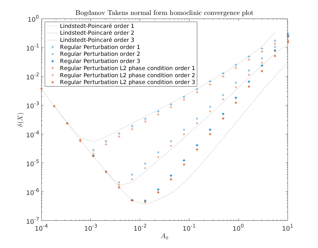
We finish this notebook with a convergence plot as above. This time we show that the \(L2\) phase-condition provides better accuracy then the phase-condition used in [AHGKM16]. However, as stated in [Kuz21] these results do not lift to the central manifold of a general system.
Also shown is that the Lindstedt-Poincaré method provides a much better approximation here then either one of the regular perturbation methods. This however doens’t hold true for the first order correction.
BToptions = BT_Hom_set_options();
BToptions.TTolerance = 1e-05;
BToptions.messages = false;
BToptions.correct = false;

amplitudes = logspace(-4, 1, 20);
methodList = {'LP', 'RegularPerturbation', 'RegularPerturbationL2'};

relativeErrors = {};
for i=1:3
    for k=1:length(methodList)
        relativeErrors{i,k} = zeros(size(amplitudes));
        BToptions.order = i;
        BToptions.method = methodList{k};
        for j=1:length(amplitudes)
            BToptions.amplitude = amplitudes(j);
            [x_pred, v0] = init_BT_Hom(odefile, bt, ap, BToptions);
            try
                x_corrected = newtcorr(x_pred, v0);
                relativeErrors{i,k}(j) = norm(x_corrected-x_pred)/norm(x_corrected);
            catch
                warning('Did not converge.')
                continue
            end
        end
    end
end

clf
cm = lines();
loglog(amplitudes, relativeErrors{1,1}(:), '-', ...
       amplitudes, relativeErrors{2,1}(:), '-', ...
       amplitudes, relativeErrors{3,1}(:), '-', ...
       amplitudes, relativeErrors{1,2}(:), '+', ...
       amplitudes, relativeErrors{2,2}(:), 'x', ...
       amplitudes, relativeErrors{3,2}(:), '*', ...
       amplitudes, relativeErrors{1,3}(:), '+', ...
       amplitudes, relativeErrors{2,3}(:), 'x', ...
       amplitudes, relativeErrors{3,3}(:), '*')
legend('Lindstedt-Poincaré order 1', 'Lindstedt-Poincaré order 2', ...
'Lindstedt-Poincaré order 3', ...
'Regular Perturbation order 1','Regular Perturbation order 2', ...
'Regular Perturbation order 3', ...
'Regular Perturbation L2 phase condition order 1', ...
'Regular Perturbation L2 phase condition order 2', ...
'Regular Perturbation L2 phase condition order 3', ...
'Location', 'NorthWest')
title('Bogdanov Takens normal form homoclinic convergence plot')
xlabel('$A_0$')
ylabel('$\delta(X)$')
ax = gca;
gray = [0.8 0.8 0.8];
ax.ColorOrder = [gray; gray; gray; cm(1,:); cm(1,:); cm(1,:); ...
                 cm(2,:); cm(2,:); cm(2,:)];
Warning: Did not converge.
