Predator-prey system with constant harvesting rate
In [BS79] the following predator-prey system with constant harvesting rate is considered
Here the parameters have the following interpretations:
\(k\) is the carrying capacity of the prey population,
\(d\) is the death rate of the predator,
\(r\) is the intrinsic growth rate of the prey population,
and \(h\) is the harvesting rate.
The function \(x \mapsto \frac{x}{e+x}\) is often called the functional response of Holling type II. The authors in [XR99] show the existence of a Bogdanov-Takens bifurcation in (4) and sketch the global bifurcation diagram including the homoclinic curve which emanates from the Bogdanov-Takens point. We study the occurrence of homoclinic orbits that emanate from the computed Bogdanov-Takens point using MatCont.
Overview
In this demo we will
Define an analytically derived Bogdanov-Takens point.
Start continuation of the homoclinic branch emanating from the Bogdanov-Takens point in two parameters \((d,h)\) using the new homoclinic smooth orbital predictor from [Kuz21].
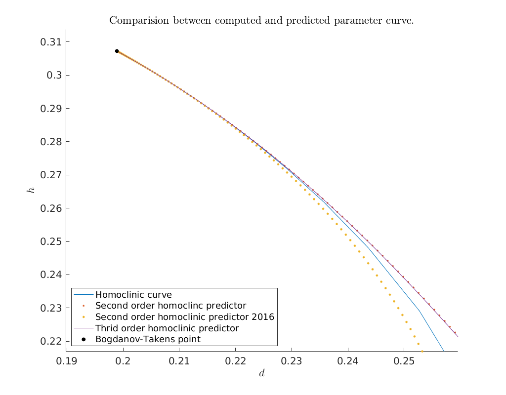
Compare the predicted and computed homoclinic bifurcation curve emanating from the Bogdanov-Takens point in parameters space.
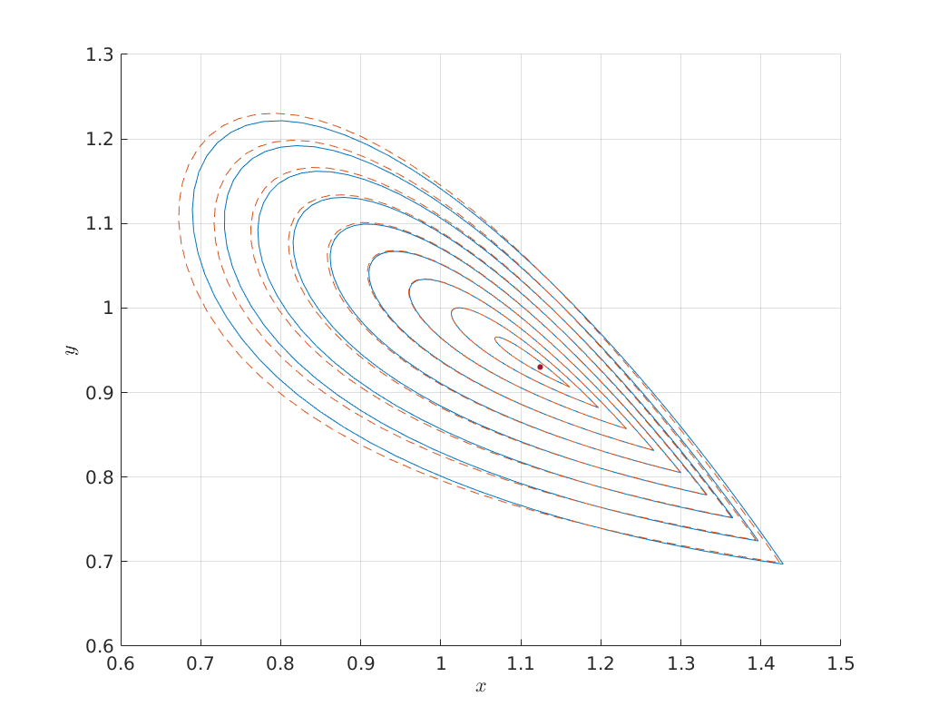
Compare a range of predictors for the homoclinic solutions emanating from the Bogdanov-Takens point with the corrected homoclinic solutions curve in phase-space.
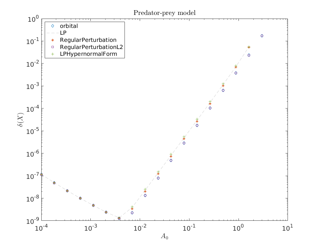
Create a convergence plot of the different homoclinic approximations derived in [Kuz21].
Load MatCont
Before we can start using MatCont we need to add the main directory of
MatCont, as well as various subdirectories of MatCont, to the MATLAB
search path. This is done in the code below. The variable matcont_home
should point to the main directory of MatCont.
clear all
matcontpath = '../';
addpath(matcontpath)
addpath([matcontpath, 'Systems'])
addpath([matcontpath, 'Equilibrium'])
addpath([matcontpath, 'LimitPoint'])
addpath([matcontpath, 'LimitPointCycle'])
addpath([matcontpath, 'Hopf'])
addpath([matcontpath, 'Homoclinic'])
addpath([matcontpath, 'LimitCycle'])
addpath([matcontpath, 'Continuer'])
addpath([matcontpath, 'MultilinearForms'])
addpath([matcontpath, 'Utilities'])
set(groot, 'defaultTextInterpreter', 'LaTeX');
set(0,'defaultAxesFontSize',15)
Set the odefile
Next we set the variable odefile to the system file previously generated by
the notebook PredatorPreyGenSym.ipynb.
odefile=@PredatorPrey;
Define Bogdanov-Takens point manually
There are two equilibrium points in (4). One is given by
By evaluating the Jacobian of (4)
at the equilibrium (5) and subsequently solving for a double zero of the characteristic equation of \(J\) for \((d,h)\) yields
d = (1/9).*(8+(-11).*(548+(-18).*894.^(1/2)).^(-1/3)+(-1).*2.^(-2/3).* ...
(274+(-9).*894.^(1/2)).^(1/3));
h = (93.*2.^(2/3)+(-9).*2.^(1/6).*447.^(1/2)+(-975).*(2.*(274+(-9).* ...
    894.^(1/2)).^(-1)).^(1/3)+36.*2.^(5/6).*447.^(1/2).*(274+(-9).* ...
    894.^(1/2)).^(-1/3)+30.*(274+(-9).*894.^(1/2)).^(1/3)).*(88.*2.^( ...
    2/3)+16.*(274+(-9).*894.^(1/2)).^(1/3)+8.*2.^(1/3).*(274+(-9).* ...
    894.^(1/2)).^(2/3)).^(-1);
x = (1/2).*((-2)+d).*((-1)+d).^(-1);
y = (1/8).*((-1)+d).^(-2).*(8+(-18).*d+9.*d.^2);
bt.x = [x; y];
bt.par = [d; h];
To refer to the parameters throughout the script we create a cell array of
strings containing the parameter names. This is then converted into a
struct. This allows us to refer to the parameters as ind.parametername,
similar as done in DDE-BifTool.
parnames = {'d', 'h'};
cind = [parnames;num2cell(1:length(parnames))];
ind  = struct(cind{:});
Continue homoclinic curve emanating from the Bogdanov-Takens point
To continue the homoclinic curve emanating from the Bogdanov-Takens point we
use the functions BT_Hom_set_options and init_BT_Hom to obtain an initial
approximation to the homoclinic solution (hom_x) as well as a tangent vector
to the discretized homoclinic solution (hom_v) as described in
Initial prediction of homoclinic orbit near Bogdanov-Takens point 1.
ap = [ind.d, ind.h];
BToptions = BT_Hom_set_options();
[hom_x, hom_v] = init_BT_Hom(odefile, bt,  ap, BToptions);
opt = contset;
opt.MaxStepsize = 5;
opt.Singularities = 0;
opt.MaxNumPoints = 200;
homoclinic_br = cont(@homoclinic, hom_x, hom_v, opt);
Center manifold coefficients' accuracy: 9.992007e-16
BT normal form coefficients:
a=1.798257e-01,	 b=-3.782866e-01
The initial perturbation parameter epsilon:  1.000000e-01
The initial amplitude: 0.0753982
The initial half-return time T: 86.8246
The initial distance eps0: 0.000144111
The initial distance eps1: 4.47679e-05
first point found
tangent vector to first point found
Current step size too small (point 118)
elapsed time  = 6.3 secs
npoints curve = 118
Compare predicted with computed parameters
Now that we have obtained a curve of homoclinic orbits (homoclinic_br) we
compare the computed curve in parameter space with the predicted curve we
construct below. To do so, we use the function BT_nmfm_orbital to obtain the
smooth orbital normal form coefficients, i.e. \(a\) and \(b\), and the coefficients
of the transformation \(K\) between the parameters of the system and the parameters
of the smooth orbital normal form on the center manifold, see
[Kuz21]. By using the transformation \(K\) as given in
[AHGKM16] where \(K_{11}\) is not included for the second order
approximation we see that including \(K_{11}\) as done in [Kuz21]
does indeed lead to a better approximation.
%plot --width 1024 --height 800
hold on
global homds
% plot computed parameter curve
plot(homoclinic_br(homds.PeriodIdx+1,:), ...
     homoclinic_br(homds.PeriodIdx+2,:));
% Bogdanov-Takens parameter-dependent normal form coefficients
bt = BT_nmfm_orbital(odefile, bt, ap, BToptions);
a   = bt.nmfm.a;
b   = bt.nmfm.b;
K10 = bt.nmfm.K10;
K01 = bt.nmfm.K01;
K02 = bt.nmfm.K02;
K11 = bt.nmfm.K11;
K03 = bt.nmfm.K03;
% construct predictor as in the paper
eps = linspace(0, 0.4);
beta1 = -4*a^3/b^4*eps.^4;
tau0  = 10/7;
tau2  = 288/2401;
beta2 = a/b*(tau0 + tau2*eps.^2).*eps.^2;
alpha = K10.*beta1 + K01.*beta2 + 1/2*K02.*beta2.^2 ...
    + K11.*beta1.*beta2 + 1/6*K03.*beta2.^3;
alphaSecondOrder = K10.*beta1 + K01.*beta2 + 1/2*K02.*beta2.^2 ...
    + K11.*beta1.*beta2;
alpha = bt.par(ap) + alpha;
alphaSecondOrder = bt.par(ap) + alphaSecondOrder;
alpha2016 = K10.*beta1 + K01.*beta2 + 1/2*K02.*beta2.^2;
alpha2016 = bt.par(ap) + alpha2016;
% plot currect predictor
plot(alphaSecondOrder(1,:), alphaSecondOrder(2,:), '.', 'MarkerSize', 7)
plot(alpha2016(1,:), alpha2016(2,:), '.', 'MarkerSize', 10)
plot(alpha(1,:), alpha(2,:), '-', 'MarkerSize', 10)
% plot Bogdanov-Takens point
plot(bt.par(ind.d), bt.par(ind.h), '.k', 'MarkerSize', 20)
% set labels and legend
xlabel('$d$')
ylabel('$h$')
legend({'Homoclinic curve', 'Second order homoclinc predictor', ...
    'Second order homoclinic predictor 2016', ...
    'Thrid order homoclinic predictor', ...
    'Bogdanov-Takens point'}, 'Location', 'SouthWest')
title('Comparision between computed and predicted parameter curve.')
axis([0.1898    0.2596    0.2169    0.3137])
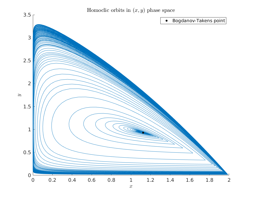
Bifurcation diagram in \((x,y)\) phase-space
To obtain an impression of the homoclinic solutions we plot the computed homoclinic orbits in \((x,y)\) phase-space.
hold on
plot(homoclinic_br(homds.coords(1:homds.nphase:end), 1:end), ...
     homoclinic_br(homds.coords(2:homds.nphase:end), 1:end), ...
     'Color', [0 0.4470 0.7410], 'HandleVisibility', 'Off')
xlabel('$x$')
ylabel('$y$')
plot(bt.x(1), bt.x(2), '.k' ,'MarkerSize', 20)
legend('Bogdanov-Takens point', 'Location', 'NorthEast')
title('Homoclic orbits in $(x,y)$ phase space')
Predictors of orbits for various epsilons
Below we compute for a large range of amplitudes the predicted and corrected
homoclinic solutions and compare them in phase space. We see that even with an
amplitude of 1 the predicted homoclinic orbit is still very close.
options = BT_Hom_set_options();
options.messages = false;
options.correct = false;
options.TTolerance = 1.0e-05;

amplitudes = linspace(1.0e-03, 1,10);
XPredicted = zeros(330,length(amplitudes));
XCorrected = zeros(330,length(amplitudes));
for j=1:length(amplitudes)
  options.amplitude = amplitudes(j);
  [x_pred, v0] = init_BT_Hom(odefile, bt, ap, options);
  XPredicted(:,j) = x_pred;
  try
    XCorrected(:,j) = newtcorr(x_pred, v0);
  catch
    warning('Didn''t convergence to homoclinic solution')
  end
end

hold on
cm = lines;
plot(XPredicted(homds.coords(1:homds.nphase:end),1:10), ...
     XPredicted(homds.coords(2:homds.nphase:end),1:10), ...
      'color', cm(1,:))
plot(XCorrected(homds.coords(1:homds.nphase:end),1:10), ...
     XCorrected(homds.coords(2:homds.nphase:end),1:10), ...
      '--', 'color', cm(2,:))
plot(bt.x(1), bt.x(2), '.', 'MarkerSize', 16)
xlabel('$x$')
ylabel('$y$')
grid on
Convergence plot
We finish this notebook with a log-log convergence plot comparing the different
third order homoclinic approximation methods derived in [Kuz21]
to approximate the homoclinic solutions near the first Bogdanov-Takens point.
On the abscissa is the amplitude \(A_0\) and on the ordinate the relative error
\(\delta\) between the constructed solution (x_pred) to the defining system for the
homoclinic orbit and the Newton corrected solution (x_corrected).
BToptions = BT_Hom_set_options();
BToptions.TTolerance = 1e-05;
BToptions.messages = false;
BToptions.correct = false;

amplitudes = logspace(-4, 1, 20);
methodList = {'orbital', 'LP', 'RegularPerturbation', ...
    'RegularPerturbationL2', 'LPHypernormalForm'};
relativeErrors = {};
for i=1:length(methodList)
    BToptions.method = methodList{i};
    relativeErrors{i} = zeros(size(amplitudes));
    for j=1:length(amplitudes)
    BToptions.amplitude = amplitudes(j);
    [x_pred, v0] = init_BT_Hom(odefile, bt, ap, BToptions);
    try
        x_corrected = newtcorr(x_pred, v0);
        relativeErrors{i}(j) = norm(x_corrected-x_pred)/norm(x_corrected);
    catch
        warning('Did not converge.')
        continue
    end
  end
end

cm = lines();
loglog(amplitudes, relativeErrors{1}(:), 'd', ...
       amplitudes, relativeErrors{2}(:), '--', ...
       amplitudes, relativeErrors{3}(:), '*', ...
       amplitudes, relativeErrors{4}(:), 's', ...
       amplitudes, relativeErrors{5}(:), '+')
legend(methodList, 'Location', 'NorthWest')
title('Predator-prey model')
xlabel('$A_0$')
ylabel('$\delta(X)$')
ax = gca;
ax.ColorOrder = [cm(1,:); [0.8 0.8 0.8]; cm(2,:); cm(4,:); cm(5,:)];
Warning: Did not converge.
Warning: Did not converge.
Warning: Did not converge.
Warning: Did not converge.
Warning: Did not converge.
Warning: Did not converge.
Warning: Did not converge.
Warning: Did not converge.
Warning: Did not converge.
Warning: Did not converge.
Warning: Did not converge.
Warning: Did not converge.
Warning: Did not converge.
