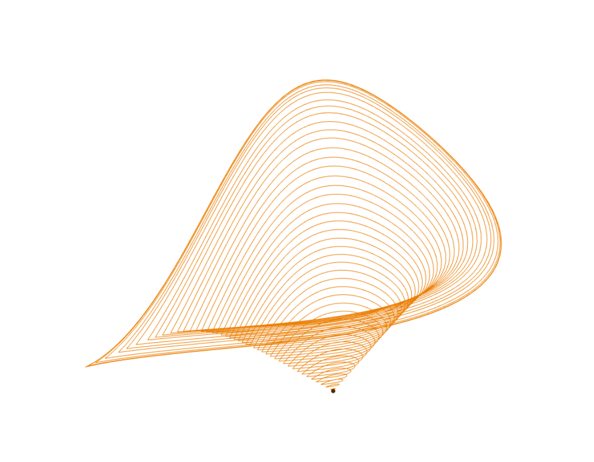
Interplay between normal forms and center manifold reduction for homoclinic predictors near Bogdanov-Takens bifurcation
In this Jupyter Book we will demonstrate the effectiveness of the homoclinic predictors derived in [Kuz21] to start continuations of homoclinic orbits in two parameters in MatCont near generic codimension two Bogdanov-Takens bifurcation points in \(n\)-dimensional ordinary differential equations (ODEs) of the form
where \(x: \mathbb R \to \mathbb R^n\) and \(\alpha \in \mathbb R^m\). The function \(f : \mathbb R^n \times \mathbb R^m \to \mathbb R^n\) is assumed to be as smooth as necessary.
In total there are eight different models considered. Each the models consists of two notebooks:
one to generate the necessary derivative files, see for example Generate system files for Morris-Lecar in a platinum model,
and one model notebook to analyse the model.
In the first two models Morris-Lecar Model, and CO-oxidation in a platinum model. we partly follow the presentation in [BAH15], that is, we define an equilibrium of (1), continue the equilibrium point one parameter, encounter a codimension one Hopf or fold bifurcation, continue the codimension one bifurcation point in two parameters and encounter one or more Bogdanov-Takens points. The homoclinic orbits emanating from these Bogdanov-Takens point can then be continued using one of the homoclinic predictors form [Kuz21] implemented into MatCont. In these first two models we will describe in detail how a homoclinic approximation near the generic codimension two Bogdanov-Takens bifurcation is obtained in MatCont.
Although the procedure described above is a common situation for discovering Bogdanov-Takens points in ODEs, in many situations it is possible to derive the Bogdanov-Takens point directly, either analytically or numerically, form the ODE. This will be the approach for the remaining models were we will focus solely on the homoclinic orbits emanating from the Bogdanov-Takens point and not the Hopf and fold curves.
At the end of each model notebook we create a convergence plot of the different methods to approximation the homoclinic solution derived in [Kuz21].
In the notebook BogdanovTakens.ipynb the importance of using a higher order approximation of the non-linear time transformation used in [Kuz21] is demonstrated.
Note
The derivative files can also be generated with the graphical user interface of MatCont. In fact, if preferred, the continuation of the various bifurcation branches can be done using only the graphical user interface.
