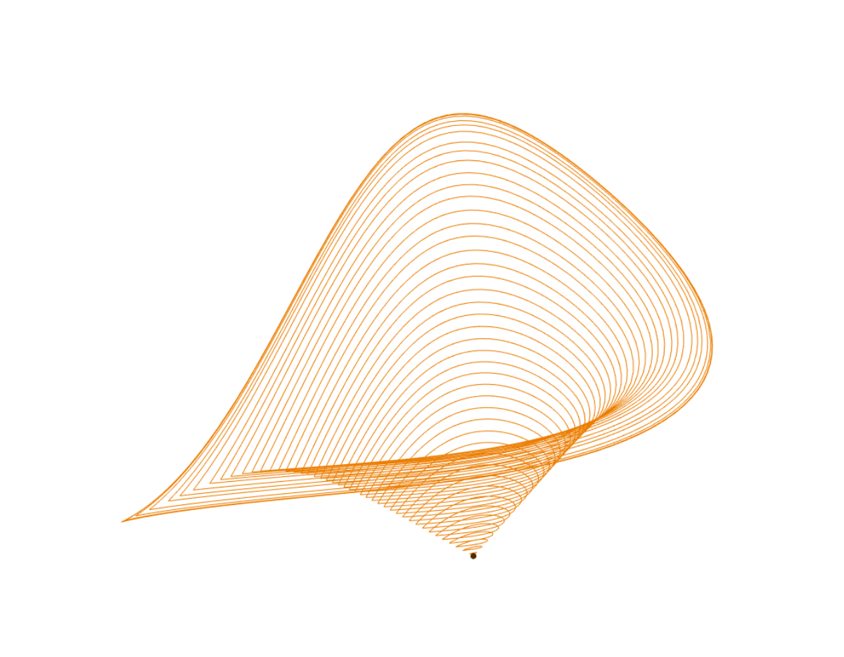
Homoclinic RG flows¶

In [JP21] an \(\mathcal{N}=1\) supersymmetric model of interacting scalar superfields that is invariant under the action of an \(O(N) \times O(M)\) group in \(d=3-\epsilon\) dimensions is considered. The coupling constants \(g_i(i=1,\dots,4)\) satisfy the following differential equations

\[ \dot g_i = -\epsilon g_i + \beta_i^{(2)}, \qquad i=1,\dots,4, \]

where the \(\beta\) functions are given by

\[\begin{split} \begin{aligned} \beta_{1}^{(2)}=& \frac{1}{8 \pi^{2} N^{2}}\left(32 g_{1}^{2} g_{4} N\left(-40-8 M+8 N+7 M N+8 N^{2}\right)+16 g_{1}^{2} g_{3} N\left(-80-24 M+30 N+4 M N+7 N^{2}+4 M N^{2}\right)\right.\\ &+16 g_{1} g_{3}^{2} N^{2}\left(32+2 M+N+M N+N^{2}+M N^{2}\right)+64 g_{1} g_{2} g_{4} N\left(-32-4 M+16 N+2 M N+5 N^{2}+2 M N^{2}\right) \\ &+4 g_{2}^{2} g_{3} N\left(-256-64 M+72 N+10 M N+19 N^{2}+2 M N^{2}\right)+64 g_{1} g_{4}^{2} N^{2}\left(22-2 M+M N+M N^{2}\right) \\ &+16 g_{1} g_{2} g_{3} N\left(-144-40 M+42 N+17 M N+21 N^{2}+5 M N^{2}\right)+128 g_{1} g_{3} g_{4} N^{2}\left(3+5 M+N+N^{2}\right) \\ &+g_{2}^{3}\left(896+128 M-352 N-48 M N-12 N^{2}-12 M N^{2}+7 N^{3}+2 M N^{3}\right)+96 g_{2}^{2} g_{4}(-8+N) N \\ &+4 g_{1}^{2} g_{2}\left(928+224 M-392 N-100 M N-2 N^{2}+11 M N^{2}+23 N^{3}+7 M N^{3}+4 N^{4}\right)+768 g_{2} g_{3} g_{4} N^{2} \\ &+4 g_{1}^{3}\left(352+96 M-152 N-44 M N+10 N^{3}+3 M N^{3}+M N^{4}\right)+16 g_{2} g_{3}^{2} N^{2}\left(16+7 M+N+N^{2}\right) \\ &\left.+2 g_{1} g_{2}^{2}\left(1600+320 M-656 N-136 M N+32 N^{2}+10 M N^{2}+50 N^{3}+10 M N^{3}+5 N^{4}+2 M N^{4}\right)\right), \end{aligned} \end{split}\]

\[\begin{split} \begin{aligned} \beta_{2}^{(2)}=& \frac{1}{8 \pi^{2} N^{2}}\left(64 g_{1} g_{2} g_{4} N\left(-80-16 M+16 N+5 M N+7 N^{2}\right)+16 g_{2} g_{3}^{2} N^{2}\left(48+9 M+2 N+M N+2 N^{2}+M N^{2}\right)\right.\\ &+16 g_{1}^{2} g_{3} N\left(-128-32 M+32 N+12 M N+14 N^{2}+3 M N^{2}\right)+128 g_{2} g_{3} g_{4} N^{2}\left(9+5 M+N+N^{2}\right) \\ &+16 g_{1} g_{2} g_{3} N\left(-272-72 M+82 N+15 M N+24 N^{2}+6 M N^{2}\right)+192 g_{1}^{2} g_{4} N\left(-12-2 M+4 N+N^{2}\right) \\ &+16 g_{2}^{2} g_{4} N\left(-176-40 M+58 N+14 M N+17 N^{2}+11 M N^{2}\right)+32 g_{1} g_{3}^{2} N^{2}\left(16+7 M+N+N^{2}\right) \\ &+4 g_{2}^{2} g_{3} N\left(-576-160 M+176 N+54 M N+74 N^{2}+17 M N^{2}\right)+64 g_{2} g_{4}^{2} N^{2}\left(22-2 M+M N+M N^{2}\right) \\ &+8 g_{1}^{3}\left(288+64 M-112 N-24 M N-6 N^{2}+3 M N^{2}+5 N^{3}+2 M N^{3}+N^{4}\right)+1536 g_{1} g_{3} g_{4} N^{2} \\ &+2 g_{1} g_{2}^{2}\left(3968+1024 M-1600 N-416 M N-56 N^{2}-22 M N^{2}+85 N^{3}+17 M N^{3}+11 N^{4}\right) \\ &+4 g_{1}^{2} g_{2}\left(1856+448 M-736 N-176 M N-22 N^{2}-5 M N^{2}+43 N^{3}+8 M N^{3}+3 N^{4}+2 M N^{4}\right) \\ &\left.+g_{2}^{3}\left(2816+768 M-1152 N-320 M N+12 N^{2}-12 M N^{2}+69 N^{3}+30 M N^{3}+7 N^{4}+5 M N^{4}\right)\right), \end{aligned} \end{split}\]

\[\begin{split} \begin{aligned} \beta_{3}^{(2)}=& \frac{1}{8 \pi^{2} N^{3}}\left(32 g_{3}^{2} g_{4} N^{3}\left(18+14 M+7 N+7 N^{2}\right)+96 g_{1}^{2} g_{4} N\left(8+2 N^{2}+M N^{2}\right)+384 g_{1} g_{2} g_{4} N\left(4+N^{2}\right)\right.\\ &+24 g_{3}^{3} N^{3}\left(16+2 M+2 N+M N+2 N^{2}+M N^{2}\right)+64 g_{2} g_{3} g_{4} N^{2}\left(-20-4 M+10 N+2 M N+5 N^{2}+2 M N^{2}\right) \\ &+16 g_{1} g_{3}^{2} N^{2}\left(-52-14 M+26 N+7 M N+14 N^{2}+7 M N^{2}\right)+128 g_{1} g_{3} g_{4} N^{2}\left(-10-2 M+5 N+M N+5 N^{2}\right) \\ &+8 g_{2} g_{3}^{2} N^{2}\left(-104-28 M+52 N+14 M N+38 N^{2}+7 M N^{2}\right)+64 g_{3} g_{4}^{2} N^{3}\left(22-2 M+M N+M N^{2}\right) \\ &+16 g_{1} g_{2} g_{3} N\left(208+56 M-48 N-12 M N+12 N^{2}+3 M N^{2}+8 N^{3}+M N^{3}+2 N^{4}\right)+96 g_{2}^{2} g 4 N\left(8+N^{2}\right) \\ &+8 g_{1}^{2} g_{3} N\left(208+56 M-48 N-12 M N+12 N^{2}+6 M N^{2}+4 N^{3}+3 M N^{3}+M N^{4}\right) \\ &+8 g_{1}^{3}\left(-96-16 M+24 N+4 M N-20 N^{2}-10 M N^{2}+6 N^{3}+2 M N^{3}+N^{4}+M N^{4}\right) \\ &+4 g_{2}^{2} g_{3} N\left(416+112 M-96 N-24 M N+18 N^{2}+6 M N^{2}+12 N^{3}+4 M N^{3}+2 N^{4}+M N^{4}\right) \\ &+g_{2}^{3}\left(-768-128 M+192 N+32 M N-96 N^{2}+32 N^{3}+4 M N^{3}+7 N^{4}+2 M N^{4}\right) \\ &+2 g_{1} g_{2}^{2}\left(-1152-192 M+288 N+48 M N-176 N^{2}-40 M N^{2}+70 N^{3}+10 M N^{3}+21 N^{4}+2 M N^{4}\right) \\ &\left.+4 g_{1}^{2} g_{2}\left(-576-96 M+144 N+24 M N-104 N^{2}-40 M N^{2}+34 N^{3}+13 M N^{3}+11 N^{4}+3 M N^{4}\right)\right), \end{aligned} \end{split}\]

and

\[\begin{split} \begin{aligned} \beta_{4}^{(2)}=& \frac{1}{8 \pi^{2} N^{3}}\left(8 g_{1}^{2} g_{3} N\left(80+16 M-12 N+4 N^{2}+2 M N^{2}+3 N^{3}+N^{4}\right)\right.\\ &+224 g_{1} g_{4}^{2} N^{2}\left(-4-2 M+2 N+M N+2 N^{2}\right)+16 g_{1} g_{3}^{2} N^{2}\left(-16-2 M+8 N+M N+7 N^{2}\right) \\ &+96 g_{4}^{3} N^{3}\left(8-2 M+M N+M N^{2}\right)+64 g_{2} g_{3} g_{4} N^{2}\left(-14-4 M+7 N+2 M N+6 N^{2}+M N^{2}\right) \\ &+224 g_{2} g_{4}^{2} N^{2}\left(-4-2 M+2 N+M N+N^{2}+M N^{2}\right)+32 g_{3}^{2} g_{4} N^{3}\left(22+N+M N+N^{2}+M N^{2}\right) \\ &+64 g_{1} g_{3} g_{4} N^{2}\left(-14-4 M+7 N+2 M N+2 N^{2}+2 M N^{2}\right) \\ &+8 g_{2} g_{3}^{2} N^{2}\left(-32-4 M+16 N+2 M N+9 N^{2}+2 M N^{2}\right)+24 g_{3}^{3} N^{3}\left(4+2 M+N+N^{2}\right) \\ &+16 g_{1} g_{2} g_{3} N\left(80+16 M-12 N+7 N^{2}+2 M N^{2}+N^{3}\right)+224 g_{3} g_{4}^{2} N^{3}\left(2 M+N+N^{2}\right) \\ &+4 g_{2}^{2} g_{3} N\left(160+32 M-24 N+17 N^{2}+7 M N^{2}+4 N^{3}+N^{4}\right) \\ &+32 g_{1} g_{2} g_{4} N\left(96+36 M-24 N-12 M N+2 N^{2}-2 M N^{2}+4 N^{3}+M N^{3}+N^{4}\right) \\ &+4 g_{1}^{3}\left(-160-48 M+40 N+12 M N+4 N^{2}+2 M N^{2}+4 N^{3}+M N^{3}+2 N^{4}\right) \\ &+2 g_{1} g_{2}^{2}\left(-960-288 M+240 N+72 M N-88 N^{2}-20 M N^{2}+39 N^{3}+7 M N^{3}+13 N^{4}\right) \\ &+16 g_{1}^{2} g_{4} N\left(96+36 M-24 N-12 M N-4 N^{2}-2 M N^{2}+2 N^{3}+3 M N^{3}+M N^{4}\right) \\ &+8 g_{1}^{2} g_{2}\left(-240-72 M+60 N+18 M N-8 N^{2}-M N^{2}+6 N^{3}+2 M N^{3}+N^{4}+M N^{4}\right) \\ &+8 g_{2}^{2} g_{4} N\left(192+72 M-48 N-24 M N+10 N^{2}+2 M N^{2}+6 N^{3}+4 M N^{3}+N^{4}+M N^{4}\right) \\ &\left.+g_{2}^{3}\left(-640-192 M+160 N+48 M N-96 N^{2}-24 M N^{2}+36 N^{3}+12 M N^{3}+10 N^{4}+5 M N^{4}\right)\right). \end{aligned} \end{split}\]

The parameter \(\epsilon\) is fixed to \(1\), while \(M\) and \(N\) are taken as unfolding parameters.

Overview¶

In this demo we will use the new homoclinic predictor from [Kuz21] to continue homoclinic curves from generic Bogdanov-Takens points. In order to do this we will:

Compute a curve of equilibria, parametrized by \(M\).
Detect various limit and Hopf points.
Start continuation from one of the detected Hopf points in two parameters \((M,N)\).
Detect two Bogdanov-Takens points.
Start continuation from the Bogdanov-Takens points in two parameters \((M,N)\).
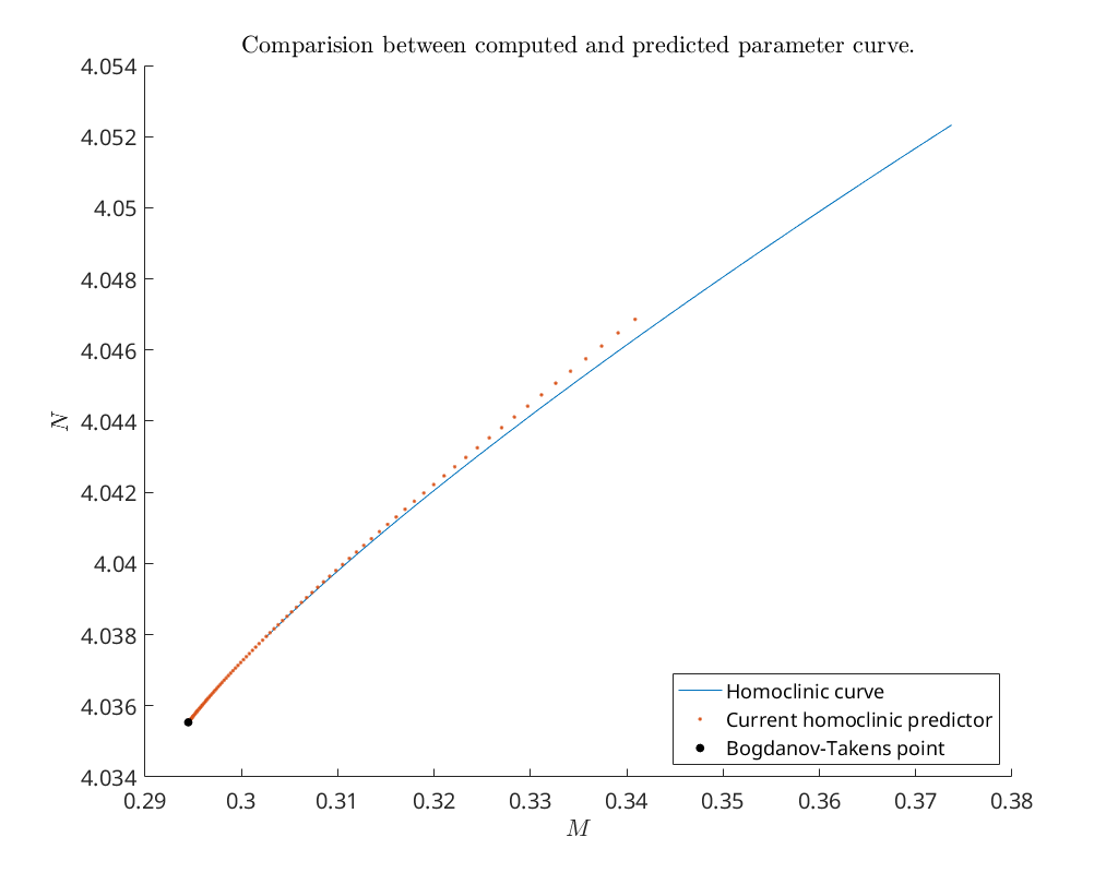
Compare the predicted and computed homoclinic bifurcation curve emanating from the first the Bogdanov-Takens point in parameters space.
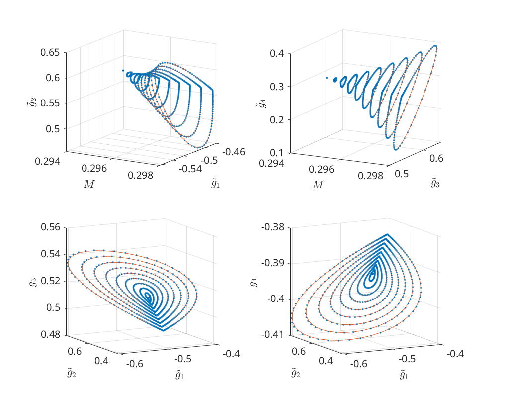
Compare a range of predictors for the homoclinic solutions emanating from the first Bogdanov-Takens point with the corrected homoclinic solutions curve in phase-space.
Create bifurcation plots including Hopf and fold curves.
Create a convergence plot comparing the different homoclinic approximations derived in [Kuz21].

Load MatCont¶

Before we can start using MatCont we need to add the main directory of MatCont, as well as various subdirectories of MatCont, to the MATLAB search path. This is done in the code below. The variable matcont_home should point to the main directory of MatCont.

clear all
matcontpath = '../';
addpath(matcontpath)
addpath([matcontpath, 'Equilibrium'])
addpath([matcontpath, 'Systems'])
addpath([matcontpath, 'Hopf'])
addpath([matcontpath, 'Homoclinic'])
addpath([matcontpath, 'LimitPoint'])
addpath([matcontpath, 'LimitCycle'])
addpath([matcontpath, 'Continuer'])
addpath([matcontpath, 'MultilinearForms'])
addpath([matcontpath, 'Utilities'])
set(groot, 'defaultTextInterpreter', 'LaTeX');
set(0,'defaultAxesFontSize',15)

Set the odefile¶

Next we set the variable odefile to the system file previously generated by the notebook HomoclinicRGflowsGenSym.ipynb.

odefile=@HomoclinicRGflows;

Define equilibrium¶

We manually define an equilibrium at

(10)¶\[(g_1, g_2, g_3, g_4) = (0.27495712275636564, 1.3931601076374327, -0.30951743797410936, -0.30951743797410936),\]

with parameter values \(M=0.2945\) and \(N = 4.036\).

To refer to the parameters throughout the script we create a cell array of strings containing the parameter names. This is then converted into a struct. This allows us to refer to the parameters as ind.parametername, similar as done in the software package DDE-BifTool [SEL+14].

parnames = {'epsilon', 'M', 'N'};
cind = [parnames;num2cell(1:length(parnames))];
ind  = struct(cind{:});
p(ind.epsilon) = 1;
p(ind.M) = 0.2945;
p(ind.N) = 4.036;
x  = [0.0701457361241472, -0.06520883770451065, 0.001823543197553845, 0.22874527306411319]';

Continue equilibrium in parameter \(N\)¶

To continue the equilibrium (10) in parameter \(N\), we first need to obtain a tangent vector to the curve. This is done by the function init_EP_EP. Then we use the function contset to obtain a struct containing a list of options which is passed on to the continuer. By adjusting the values of the fields of the opt struct we set the maximum step size. We also set the maximum number of points to continue and weather or not to detect bifurcation points (opt.Singularities) on the equilibrium curve. For more information about all options available to the MatCont continuer and the continuation process in general, we refer to [DGK+08].

Finally, we continue the curve using the function cont.

[x1_pred, v1_pred] = init_EP_EP(odefile, x, p, ind.M);
opt = contset;
opt.MaxNumPoints  = 300;
opt.Singularities = 1;
opt.Backward = 1;
[eqbr_x, ~, eqbr_bif_data] = cont(@equilibrium, x1_pred, v1_pred, opt);

first point found
tangent vector to first point found
Neutral saddle
label = H , x = ( 0.000002 -0.000003 -0.000000 0.171390 1.091355 )
label = LP, x = ( -0.110189 0.142208 0.003572 0.100776 1.998164 )
a=-7.331116e-01
Neutral saddle
label = H , x = ( -0.579707 0.570669 0.013951 -0.019833 0.966823 )
label = LP, x = ( -0.876594 0.748784 0.043787 -0.092572 0.823874 )
a=3.488423e+00
Neutral saddle
label = H , x = ( -0.945788 0.778645 0.058703 -0.115668 0.837025 )
Neutral saddle
label = H , x = ( -0.990782 0.796522 0.076078 -0.141243 0.873995 )
label = LP, x = ( -1.273488 1.256015 0.469461 -0.638409 1.000164 )
a=7.585356e-01
label = LP, x = ( -1.345207 1.354790 0.724609 -0.959767 0.979759 )
a=-8.763553e-01
Neutral saddle
label = H , x = ( -1.042702 1.041690 0.603050 -0.814403 0.981600 )
label = BP, x = ( -0.541043 0.530513 0.349786 -0.520872 1.001623 )
label = BP, x = ( -0.541043 0.530513 0.349786 -0.520872 1.001623 )
Neutral saddle
label = H , x = ( -0.118398 0.237762 0.080743 -0.300349 1.024672 )
label = LP, x = ( -0.009751 0.027361 0.006892 -0.184779 1.098410 )
a=4.606024e-02
Warning: Matrix is close to singular or badly scaled. Results may be inaccurate. RCOND =  1.832631e-16.
> In equilibrium>locateBP (line 300)
In equilibrium>locate (line 214)
In cont (line 454)

Warning: Matrix is close to singular or badly scaled. Results may be inaccurate. RCOND =  1.671679e-16.
> In equilibrium>locateBP (line 300)
In equilibrium>locate (line 214)
In cont (line 454)

Warning: Matrix is close to singular or badly scaled. Results may be inaccurate. RCOND =  1.796148e-16.
> In equilibrium>locateBP (line 300)
In equilibrium>locate (line 214)
In cont (line 454)

Warning: Matrix is close to singular or badly scaled. Results may be inaccurate. RCOND =  6.596977e-17.
> In equilibrium>locateBP (line 300)
In equilibrium>locate (line 214)
In cont (line 454)

Warning: Matrix is close to singular or badly scaled. Results may be inaccurate. RCOND =  9.044303e-18.
> In equilibrium>locateBP (line 300)
In equilibrium>locate (line 214)
In cont (line 454)

Neutral saddle
label = H , x = ( 0.000004 -0.000012 -0.000003 -0.171382 1.091381 )
label = LP, x = ( 0.082791 -0.165490 -0.069470 -0.123735 0.030515 )
a=1.327431e+00
Neutral saddle
label = H , x = ( 0.017075 -0.016965 -0.013449 -0.162484 1.015832 )
Neutral saddle
label = H , x = ( 0.000034 -0.000033 -0.000027 -0.171369 1.091270 )
label = LP, x = ( -0.057200 0.053194 0.043292 -0.205042 1.166392 )
a=1.588963e-01
label = H , x = ( -1.161474 -0.089034 0.877004 -0.621034 0.674701 )
First Lyapunov coefficient = 4.229695e-01
label = H , x = ( -0.720879 -0.252515 0.514609 -0.394150 0.295843 )
First Lyapunov coefficient = -3.941504e+00
label = LP, x = ( -0.712373 -0.249398 0.507987 -0.391094 0.295815 )
a=-6.258319e+02
Neutral saddle
label = H , x = ( -0.386826 -0.127182 0.261001 -0.280979 0.367126 )
label = LP, x = ( 0.065249 0.011257 -0.036715 -0.160519 1.196516 )
a=-2.872173e-01
Neutral saddle
label = H , x = ( 0.648955 0.299168 -0.444774 -0.280762 -1.007194 )

elapsed time  = 1.0 secs
npoints curve = 300

There are multiple Hopf (H) and limit bifurcation points detected (LP). The array struct eqbr_bif_data contains information about the detected bifurcation points. We use this to extract the index of the detected bifurcation points on the equilibrium curve eqbr_x. The equilibrium curve eqbr_x is just a two dimensional array. Each column consists of a point on the curve. The first four rows contain the point \(g\) while the last row contains the parameter \(M\).

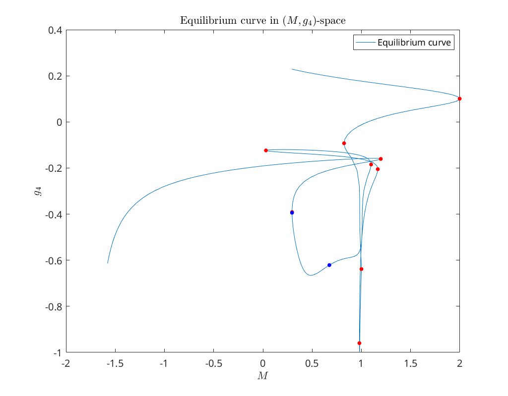
Below we plot the equilibrium curve eqbr_x, together with the detected Hopf and limit points, in \((M,g_4)\)-space.

%plot --width 1024 --height 800
plot(eqbr_x(5,:), eqbr_x(4,:)); hold on
foldInfo   = eqbr_bif_data(strcmp({eqbr_bif_data.msg}, 'Limit point')==1);
foldInfocell = struct2cell(foldInfo);
foldInd = cell2mat(foldInfocell(1,:));
hopfInfo   = eqbr_bif_data(strcmp({eqbr_bif_data.msg}, 'Hopf')==1);
hopfInfocell = struct2cell(hopfInfo);
hopfInd = cell2mat(hopfInfocell(1,:));
plot(eqbr_x(5,foldInd), eqbr_x(4,foldInd), '.r', 'MarkerSize', 20); hold on
plot(eqbr_x(5,hopfInd), eqbr_x(4,hopfInd), '.b', 'MarkerSize', 20); hold on
xlabel('$M$')
ylabel('$g_4$')
legend({'Equilibrium curve'}, 'Location', 'NorthEast')
title('Equilibrium curve in $(M,g_4)$-space')

Setup Hopf point¶

To continue the first Hopf point detected on the equilibrium branch eqbr_x in the parameters \(M\) and \(N\) we construct a new point Hopf containing the position and parameter values. These are needed to obtain an initial tangent vector - using the function init_H_H - in the full phase/parameter space. Since, from now on, we will be using the continuation parameters \(M\) and \(N\) frequently we assigned these parameters to the variable ap (active parameters).

ap = [ind.M ind.N];
hopfInfo = eqbr_bif_data(strcmp({eqbr_bif_data.msg}, 'Hopf')==1);
hopf.x = eqbr_x(1:4,hopfInfo(2).index);
hopf.par = p';
hopf.par(ind.M) = eqbr_x(5,hopfInfo(2).index);
[hopf1_x, hopf1_v] = init_H_H(odefile, hopf.x, hopf.par, ap);

Continue Hopf point in parameters \(M\) and \(N\)¶

We continue the Hopf point curve using again the function cont. We use the same continuation options as before defined above in the struct opt, but set additionally the following options. We increase the number of maximum allowed continuation points. We also increase the accuracy for locating detected bifurcations (TestTolerance) and the maximum number of iterations that may be used to achieve this (MaxTestIters). This improves the homoclinic predictor which depend directly on the accuracy of the located Bogdanov-Takens point.

opt.TestTolerance = 1e-12;
opt.MaxTestIters = 10;
opt.Backward = 0;
opt.MaxNumPoints = 50;
[hopf_br, ~, hopf_br_bif] = cont(@hopf, hopf1_x, hopf1_v, opt);

first point found
tangent vector to first point found
label = BT, x = ( -0.715157 -0.250968 0.510051 -0.391935 0.294477 4.035536 0.000000 )
(a,b)=(1.387256e+00, -1.894680e-01)
label = HH, x = ( -0.642016 -0.228678 0.452440 -0.364578 0.283522 4.030314 -0.291003 )
Neutral saddle ?
label = BT, x = ( -0.133317 0.022458 0.090992 -0.220100 0.883754 4.419949 0.000000 )
(a,b)=(-2.411266e-02, -5.207995e-01)
label = BT, x = ( -0.132423 0.106649 0.089399 -0.248054 0.942195 4.593759 -0.000000 )
(a,b)=(-7.110064e-03, 5.333636e-02)
label = HH, x = ( -0.410202 0.398065 0.256144 -0.441341 0.950248 4.384951 -0.038318 )
Neutral saddle ?

elapsed time  = 0.6 secs
npoints curve = 50

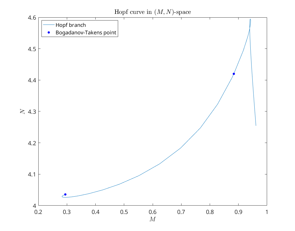
There are two Bogdanov-Takens bifurcation points (BT) detected on the limit point branch lp_br.

As with the limit points, information about the detected bifurcation points is stored in the struct array lp_br_bif. Below we extract the Bogdanov-Takens bifurcation points.

bt_points_info = hopf_br_bif(strcmp({hopf_br_bif.label}, 'BT')==1);
BTPoint1 = hopf_br(:,bt_points_info(1).index);
BTPoint2 = hopf_br(:,bt_points_info(2).index);
plot(hopf_br(5,:), hopf_br(6,:)); hold on
plot(BTPoint1(5), BTPoint1(6), '.b' ,'MarkerSize', 20)
plot(BTPoint2(5), BTPoint2(6), '.b' ,'MarkerSize', 20)
xlabel('$M$')
ylabel('$N$')
legend({'Hopf branch', 'Bogadanov-Takens point'}, 'Location', 'NorthWest')
title('Hopf curve in $(M,N)$-space')

Initial prediction of homoclinic orbit near Bogdanov-Takens point 1¶

To obtain an initial approximation to the homoclinic solution near the Bogdanov-Takens point we use the function init_BT_Hom. Its arguments are the system file (odefile), the Bogdanov-Takens point (bt1) as defined below, the unfolding parameters (ap) and an options structure (BToptions). The options structure created with the function BT_Hom_set_options contains the following fields:

ntst Number of mesh intervals with a default value of 40.
ncol Number of collocation points used in each interval with a default of 4.
extravec Three dimensional boolean row vector indicating which homoclinic parameters are selected to be free. The first component refers to the half-return time, while the second and third components refer to the distances from the saddle point to the first, respectively, the last point on the homoclinic orbit. The default value is set to [0 1 1]. Thus, the half-return time T is fixed.
order The order of the homoclinic approximation used with a default value of 3.
amplitude Desired amplitude of the homoclinic solution. If left empty then a conservative estimate is made, see [Kuz21].
TTolerance Desired distance between the last point on the numerical homoclinic solution and the saddle point. This should be at least be smaller than the amplitude. If left empty it is defined by amplitude*1.0e-03.
HigherOrderTimeReparametrization Boolean to indicate if a higher order approximation to the nonlinear time transformation in the Lindstedt-Poincaré method should be used. This should always be set to 1. It is only implemented for demonstration purposes.
method Selects the method to be used to approximate the homoclinic solution. The different methods available are:
- orbital (the default),
- orbitalv2,
- LP (Lindstedt-Poincaré with smooth normal form),
- LPHypernormalForm,
- RegularPerturbation,
- RegularPerturbationL2.
We refer to [Kuz21] for the interpretations.
messages Boolean to indicate if information about selected parameter should be printed the console. The default value is set to true.
correct Boolean to indicate if the predicted homoclinic solution should be corrected with Newton. The default value is set to true.

Here we will use most of of default values for the Bogdanov-Takens option structure. We set the field correct to false and manually correct the approximation. Also, we set the field amplitude to 0.2 to start continuation closer to the Bogdanov-Takens point. This looks better in the bifurcation diagram below. However, if we do not set the field amplitiude convergence is achived aswell.

bt_index = bt_points_info(1).index;
bt1.x = hopf_br(1:4, bt_index);
bt1.par = p';
bt1.par(ap) = hopf_br(5:6, bt_index);
BToptions = BT_Hom_set_options();
BToptions.correct = false;
BToptions.amplitude = 0.2;
[x1_pred, v1_pred] = init_BT_Hom(odefile, bt1, ap, BToptions);

Center manifold coefficients' accuracy: 7.730705e-12
BT normal form coefficients:
a=1.387256e+00,	 b=-1.894680e-01
The initial perturbation parameter epsilon:  2.936952e-02
The initial amplitude: 0.2
The initial half-return time T: 19.6487
The initial distance eps0: 0.000170201
The initial distance eps1: 0.000126381

Correct initial prediction of homoclinic orbit near bt1 with Newton¶

Now that we have an initial prediction for the homoclinic orbit we manually correct it using Newton. After the homoclinic predictor is corrected with the MatCont function newtcorr we use the function bt_rearr (Bogdanov-Takens rearrange) to extract the homoclinic orbit and saddle point from the homoclinic correction.

[hom1_x, hom1_v, ~] = newtcorr(x1_pred, v1_pred);
[x1_orbit, x1_saddle] = bt_rearr(hom1_x);

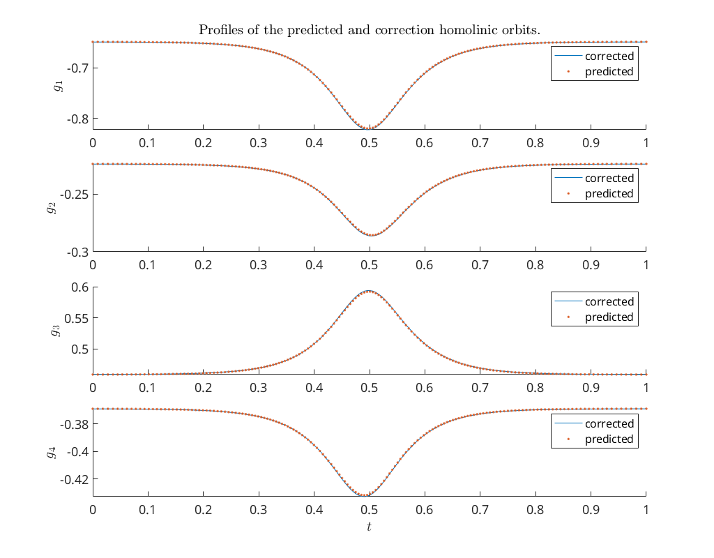
Compare profiles of predicted and corrected solution (bt1)¶

Using again the MatCont function bt_rearr, but now on the homoclinic prediction x1_pred we compare the profiles of the predicted and corrected homoclinic orbits. We see that they are indistinguishable. Note that to access the mesh on which the homoclinic orbit is computed we need the global variable homds.

[homoclinic1_pred, saddle1_pred] = bt_rearr(x1_pred);
subplot(4,1,1); hold on;
global homds
title('Profiles of the predicted and correction homolinic orbits.')
plot(homds.finemsh, x1_orbit(1:4:end))
plot(homds.finemsh, homoclinic1_pred(1:4:end),'.')
legend({'corrected', 'predicted'})
ylabel('$g_1$')
subplot(4,1,2); hold on;
plot(homds.finemsh, x1_orbit(2:4:end))
plot(homds.finemsh, homoclinic1_pred(2:4:end),'.')
legend({'corrected','predicted'})
ylabel('$g_2$')
subplot(4,1,3); hold on;
plot(homds.finemsh, x1_orbit(3:4:end))
plot(homds.finemsh, homoclinic1_pred(3:4:end),'.')
legend({'corrected','predicted'})
ylabel('$g_3$')
subplot(4,1,4); hold on;
plot(homds.finemsh, x1_orbit(4:4:end))
plot(homds.finemsh, homoclinic1_pred(4:4:end),'.')
legend({'corrected','predicted'})
ylabel('$g_4$')
legend({'corrected',  'predicted'})
xlabel('$t$')

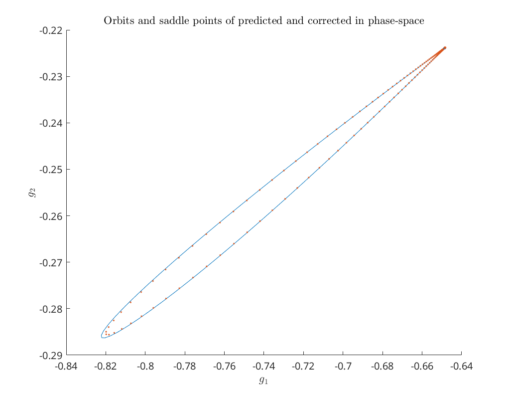
Compare predictor and corrected solution in \((g_1, g_2)\) phase-space¶

Below we compare the predicted and corrected homoclinic orbit in \((g_1, g_2)\) phase-space, as well as the predicted and corrected saddle point.

hold on
plot(x1_orbit(1:4:end),x1_orbit(2:4:end))
plot(homoclinic1_pred(1:4:end),homoclinic1_pred(2:4:end),'.')
plot(x1_saddle(1), x1_saddle(2),'.', 'MarkerSize', 12, 'Color', [0 0.4470 0.7410])
plot(saddle1_pred(1), saddle1_pred(2),'.', 'MarkerSize', 12, 'Color', [0.8500, 0.3250, 0.0980])
xlabel('$g_1$')
ylabel('$g_2$')
title('Orbits and saddle points of predicted and corrected in phase-space')

Continue homoclinic curve emanating from the first Bogdanov-Takens point¶

Having obtain an initial approximation [hom_x, hom_v], where homo_v is the tangent vector to the homoclinic curve pointing outwards from the Bogdanov-Takens point, we can start continuation using the function cont.

[homoclinic_br1, homoclinic_br1_v, homoclinic_singularities] = cont(@homoclinic, hom1_x, hom1_v, opt);

first point found
tangent vector to first point found
Inclination-flip with respect to the unstable manifold, parameters = 0.32798 and 4.04374.

elapsed time  = 9.2 secs
npoints curve = 50

Compare predicted with computed parameters emanating from bt1¶

Now that we have obtained a curve of homoclinic orbits (homoclinic_br) we compare the computed curve in parameter space with the predicted curve we construct below. To do so, we use the function BT_nmfm_orbital to obtain the smooth orbital normal form coefficients, i.e. \(a\) and \(b\), and the coefficients of the transformation \(K\) between the parameters of the system and the parameters in the smooth orbital normal form, see [Kuz21].

hold on
% plot computed homoclinic parameter curve
plot(homoclinic_br1(homds.PeriodIdx+1,:), ...
     homoclinic_br1(homds.PeriodIdx+2,:));
% Bogdanov-Takens parameter-dependent smooth orbital normal form coefficients
bt1 = BT_nmfm_orbital(odefile, bt1, ap, BToptions);
a   = bt1.nmfm.a;
b   = bt1.nmfm.b;
K10 = bt1.nmfm.K10;
K01 = bt1.nmfm.K01;
K02 = bt1.nmfm.K02;
K11 = bt1.nmfm.K11;
K03 = bt1.nmfm.K03;
% construct predictor as in the paper
eps = linspace(0, 0.05);
beta1 = -4*a^3/b^4*eps.^4;
tau0  = 10/7;
tau2  = 288/2401;
beta2 = a/b*(tau0 + tau2*eps.^2).*eps.^2;
alpha = K10.*beta1 + K01.*beta2 + 1/2*K02.*beta2.^2 ...
    + K11.*beta1.*beta2 + 1/6*K03.*beta2.^3;
alpha = bt1.par(ap) + alpha;
% plot currect predictor
plot(alpha(1,:), alpha(2,:), '.')
% plot Bogdanov-Takens point
plot(bt1.par(ind.M), bt1.par(ind.N), '.k', 'MarkerSize', 20)
% set axis labels and legend
xlabel('$M$')
ylabel('$N$')
legend({'Homoclinic curve', 'Current homoclinic predictor', ...
    'Bogdanov-Takens point'}, 'Location', 'SouthEast')
title('Comparision between computed and predicted parameter curve.')

Center manifold coefficients' accuracy: 7.730705e-12

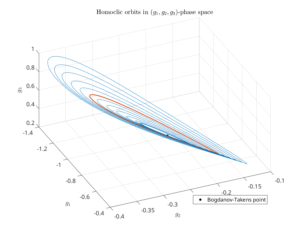
Bifurcation diagram in \((g_1,g_2,g_3)\) phase-space¶

To obtain an impression of the homoclinic solutions we plot the computed homoclinic orbits in \((g_1,g_2,g_3)\) phase-space. The red curve is the singularities detected on the homoclinic branch.

global homds
cm = lines;
hold on
plot3(homoclinic_br1(homds.coords(1:homds.nphase:end), 1:4:end), ...
      homoclinic_br1(homds.coords(2:homds.nphase:end), 1:4:end), ...
      homoclinic_br1(homds.coords(3:homds.nphase:end), 1:4:end), ...
      'Color', cm(1,:), 'HandleVisibility', 'Off')
bif_points = struct2cell(homoclinic_singularities);
plot3(homoclinic_br1(homds.coords(1:homds.nphase:end), cell2mat(bif_points(1,2:end-1))), ...
      homoclinic_br1(homds.coords(2:homds.nphase:end), cell2mat(bif_points(1,2:end-1))), ...
      homoclinic_br1(homds.coords(3:homds.nphase:end), cell2mat(bif_points(1,2:end-1))), ...
      'Color', cm(2,:), 'HandleVisibility', 'Off', 'LineWidth', 2)
xlabel('$g_1$')
ylabel('$g_2$')
zlabel('$g_3$')
plot3(bt1.x(1), bt1.x(2), bt1.x(3), '.k' ,'MarkerSize', 20)
legend('Bogdanov-Takens point', 'Location', 'SouthEast')
title('Homoclic orbits in $(g_1,g_2,g_3)$-phase space')
grid on
view(66, 50) 

Predictors of orbits for various epsilons¶

Before proceeding with continuing the homoclinic orbits emanating from the remaining three Bogdanov-Takens points we show that the estimate of the amplitude is very conservative. Below we compute for a large range of amplitudes the predicted and corrected homoclinic solutions and compare them in phase space. We see that for amplitudes up to 1.0e-02 the predicted homoclinic orbits are indistinguishable.

options = BT_Hom_set_options();
options.messages = false;
options.correct = false;
options.TTolerance = 1.0e-05;

amplitudes = linspace(1.0e-03, 1.0e-01, 10);
XPredicted = zeros(660,length(amplitudes));
XCorrected = zeros(660,length(amplitudes));
for j=1:length(amplitudes)
  options.amplitude = amplitudes(j);
  [x_pred, v0] = init_BT_Hom(odefile, bt1, ap, options);
  XPredicted(:,j) = x_pred;
  try
    XCorrected(:,j) = newtcorr(x_pred, v0);
  catch
    warning('Didn''t convergence to homoclinic solution')
  end
end

clf
subplot(2,2,1); hold on
R = @(alpha) [cos(alpha) -sin(alpha); sin(alpha) cos(alpha)];
S = @(s) [s 0; 0 1];
parsCorrected = XCorrected(homds.PeriodIdx+1,1:end).*ones(homds.tps,10);
for i=1:length(amplitudes)
    [profile, saddle] = bt_rearr(XCorrected(:,i));
    profile = reshape(profile,4,[]);
    profileRotated = R(-1.2181)*(S(100)*R(1.2181)*(profile(1:2,:) ...
                        - saddle(1:2)) + saddle(1:2));
    plot3(parsCorrected(:,i),profileRotated(1,:)', profileRotated(2,:)', ...
          '.','color', cm(1,:))

    [profile, saddle] = bt_rearr(XPredicted(:,i));
    profile = reshape(profile,4,[]);
    profileRotated = R(-1.2181)*(S(100)*R(1.2181)*(profile(1:2,:) ...
                        - saddle(1:2)) + saddle(1:2));
    plot3(parsCorrected(:,i),profileRotated(1,:)', profileRotated(2,:)', ...
          'color', cm(2,:))
end
xlabel('$M$')
ylabel('$\tilde g_1$')
zlabel('$\tilde g_2$')
grid on
view(32,15)

subplot(2,2,2); hold on
for i=1:length(amplitudes)
    alpha0 = -1.139;
    [profile, saddle] = bt_rearr(XCorrected(:,i));
    profile = reshape(profile,4,[]);
    profileRotated = R(-alpha0)*(S(100)*R(alpha0)*(profile(3:4,:) ...
                        - saddle(3:4)) + saddle(3:4));
    plot3(parsCorrected(:,i),profileRotated(1,:)', profileRotated(2,:)', ...
          '.','color', cm(1,:))

    [profile, saddle] = bt_rearr(XPredicted(:,i));
    profile = reshape(profile,4,[]);
    profileRotated = R(-alpha0)*(S(100)*R(alpha0)*(profile(3:4,:) ...
                        - saddle(3:4)) + saddle(3:4));
    plot3(parsCorrected(:,i),profileRotated(1,:)', profileRotated(2,:)', ...
          'color', cm(2,:))
end
xlabel('$M$')
ylabel('$\tilde g_3$')
zlabel('$\tilde g_4$')
grid on
view(28,15)

subplot(2,2,3); hold on
R = @(alpha) [cos(alpha) -sin(alpha) 0; sin(alpha) cos(alpha) 0; 0 0 1];
S = @(s) [s 0 0; 0 1 0; 0 0 1];
for i=1:length(amplitudes)
    [profile, saddle] = bt_rearr(XCorrected(:,i));
    profile = reshape(profile,4,[]);
    profileRotated = R(-1.2181)*(S(200)*R(1.2181)*(profile(1:3,:) ...
                        - saddle(1:3)) + saddle(1:3));
    plot3(profileRotated(1,:)', profileRotated(2,:)', profileRotated(3,:)', ...
          '.','color', cm(1,:))

    [profile, saddle] = bt_rearr(XPredicted(:,i));
    profile = reshape(profile,4,[]);
    profileRotated = R(-1.2181)*(S(200)*R(1.2181)*(profile(1:3,:) ...
                        - saddle(1:3)) + saddle(1:3));
    plot3(profileRotated(1,:)', profileRotated(2,:)', profileRotated(3,:)', ...
          'color', cm(2,:))
end
xlabel('$\tilde g_1$')
ylabel('$\tilde g_2$')
zlabel('$g_3$')
grid on
view(332,11)

subplot(2,2,4); hold on
for i=1:length(amplitudes)
    [profile, saddle] = bt_rearr(XCorrected(:,i));
    profile = reshape(profile,4,[]);
    profileRotated = R(-1.2181)*(S(200)*R(1.2181)*(profile([1,2,4],:) ...
                        - saddle([1,2,4])) + saddle([1,2,4]));
    plot3(profileRotated(1,:)', profileRotated(2,:)', profileRotated(3,:)', ...
          '.','color', cm(1,:))

    [profile, saddle] = bt_rearr(XPredicted(:,i));
    profile = reshape(profile,4,[]);
    profileRotated = R(-1.2181)*(S(200)*R(1.2181)*(profile([1,2,4],:) ...
                        - saddle([1,2,4])) + saddle([1,2,4]));
    plot3(profileRotated(1,:)', profileRotated(2,:)', profileRotated(3,:)', ...
          'color', cm(2,:))
end
xlabel('$\tilde g_1$')
ylabel('$\tilde g_2$')
zlabel('$g_4$')
grid on
view(332,11)

Continue limit points emanating from the Bogdanov-Takens point¶

Next we also continue the limit points emanating from the Bogdanov-Takens points.

[lp1_x, lp1_v] = init_BT_LP(odefile, bt1.x, bt1.par, ap);
[lp_br, ~, lp_br1_bif] = cont(@limitpoint, lp1_x, lp1_v, opt);
opt.Backward = 1;
lp_br_rev = cont(@limitpoint, lp1_x, lp1_v, opt);

first point found
tangent vector to first point found
label = BT, x = ( -0.133317 0.022458 0.090992 -0.220100 0.883754 4.419949 )
(a,b)=(-2.411266e-02, -5.207995e-01)
Warning: Matrix is close to singular or badly scaled. Results may be inaccurate. RCOND =  1.198603e-16.
> In limitpoint>curve_func (line 26)
In newtcorr (line 21)
In cont (line 358)

Warning: Matrix is close to singular or badly scaled. Results may be inaccurate. RCOND = 4.557903e-114.
> In limitpoint>curve_func (line 26)
In newtcorr (line 21)
In cont (line 358)

Warning: Matrix is singular, close to singular or badly scaled. Results may be inaccurate. RCOND = NaN.
> In limitpoint>curve_func (line 26)
In newtcorr (line 21)
In cont (line 358)

label = CP, x = ( -0.068275 0.012534 0.046191 -0.194560 0.905065 4.487600 )
c=1.231052e+00
Warning: Matrix is close to singular or badly scaled. Results may be inaccurate. RCOND =  2.445239e-19.
> In limitpoint>curve_func (line 26)
In newtcorr (line 21)
In cont>LocateTestFunction (line 945)
In cont (line 465)

Warning: Matrix is close to singular or badly scaled. Results may be inaccurate. RCOND = 3.462497e-125.
> In limitpoint>curve_func (line 26)
In newtcorr (line 21)
In cont>LocateTestFunction (line 945)
In cont (line 465)

Warning: Matrix is singular, close to singular or badly scaled. Results may be inaccurate. RCOND = NaN.
> In limitpoint>curve_func (line 26)
In newtcorr (line 21)
In cont>LocateTestFunction (line 945)
In cont (line 465)

label = ZH, x = ( 0.089558 0.013324 -0.045799 -0.157071 1.383946 3.902668 )
Neutral saddle
Zero-Neutral Saddle

elapsed time  = 0.3 secs
npoints curve = 50
first point found
tangent vector to first point found
label = BT, x = ( -0.715157 -0.250968 0.510051 -0.391935 0.294477 4.035536 )
(a,b)=(-1.387256e+00, 1.894680e-01)

elapsed time  = 0.1 secs
npoints curve = 50

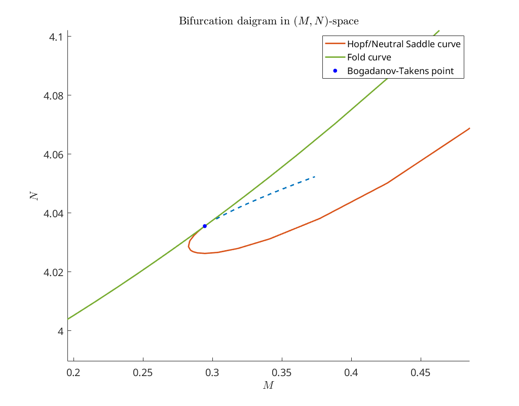
We see that there are two additional Bogdanov-Takens points detected.

Bifurcation plot¶

Next we plot the continued curves in \((M,N)\) parameter space near the first Bogdanov-Takens point.

%plot inline 
hold on
homColor  = cm(1,:);
hopfColor = cm(2,:);
foldColor = cm(5,:);
plot(hopf_br(5,:), hopf_br(6,:), 'Color', hopfColor, 'linewidth', 2)
plot(lp_br(5,:), lp_br(6,:), 'Color', foldColor, 'linewidth', 2)
plot(lp_br_rev(5,:), lp_br_rev(6,:), 'Color', foldColor, 'linewidth', 2, ...
    'HandleVisibility', 'Off', 'linewidth', 2);
plot(BTPoint1(5), BTPoint1(6), '.b' ,'MarkerSize', 20)
plot(homoclinic_br1(homds.PeriodIdx+1,:), ...
     homoclinic_br1(homds.PeriodIdx+2,:), ...
     '--', 'Color', homColor, 'linewidth', 2, 'HandleVisibility', 'Off')
xlabel('$M$')
ylabel('$N$')
legend({'Hopf/Neutral Saddle curve', 'Fold curve',...
    'Bogadanov-Takens point'}, 'Location', 'NorthEast')
title('Bifurcation daigram in $(M,N)$-space')
axis([0.1956    0.4852    3.9896    4.1020])

Convergence plot¶

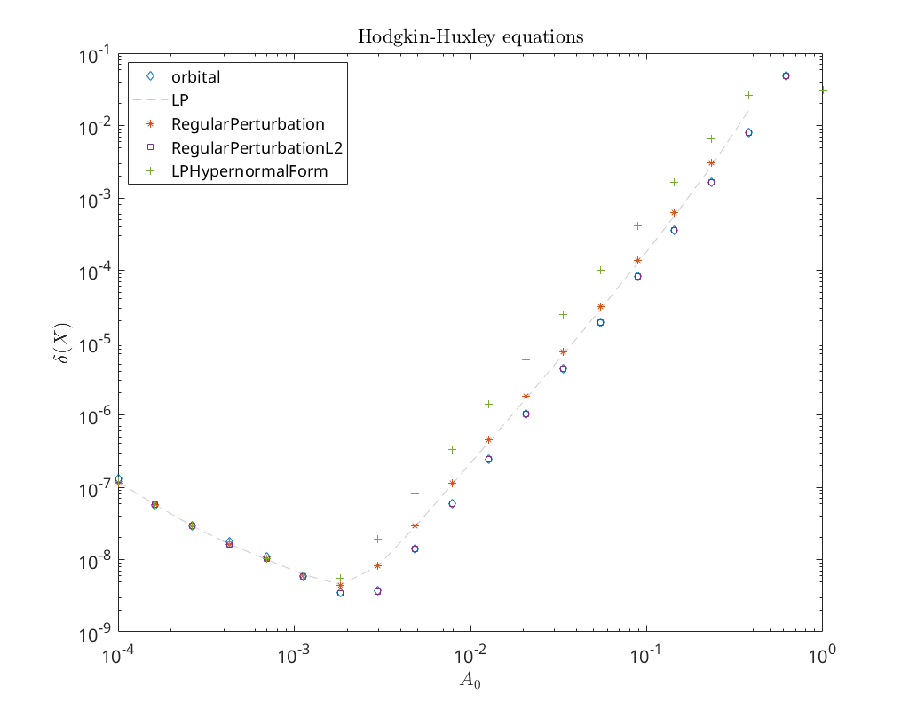
We finish this notebook with a log-log convergence plot comparing the different third order homoclinic approximation methods derived in [Kuz21] to approximate the homoclinic solutions near the first Bogdanov-Takens point. On the abscissa is the amplitude \(A_0\) and on the ordinate the relative error \(\delta\) between the constructed solution (x_pred) to the defining system for the homoclinic orbit and the Newton corrected solution (x_corrected).

BToptions = BT_Hom_set_options();
BToptions.TTolerance = 1e-05;
BToptions.messages = false;
BToptions.correct = false;

amplitudes = logspace(-4, 0, 20);
methodList = {'orbital', 'LP', 'RegularPerturbation', ...
    'RegularPerturbationL2', 'LPHypernormalForm'};
relativeErrors = {};
for i=1:length(methodList)
    for o=1:3
        BToptions.method = methodList{i};
        BToptions.order = o;
        relativeErrors{o,i} = zeros(size(amplitudes));
        for j=1:length(amplitudes)
            BToptions.amplitude = amplitudes(j);
            [x_pred, v0] = init_BT_Hom(odefile, bt1, ap, BToptions);
            try
                x_corrected = newtcorr(x_pred, v0);
                relativeErrors{o,i}(j) = norm(x_corrected-x_pred)/norm(x_corrected);
            catch
                warning('Did not converge.')
                continue
            end
        end
    end
end

cm = lines();
loglog(amplitudes, relativeErrors{3,1}(:), 'd', ...
       amplitudes, relativeErrors{3,2}(:), '--', ...
       amplitudes, relativeErrors{3,3}(:), '*', ...
       amplitudes, relativeErrors{3,4}(:), 's', ...
       amplitudes, relativeErrors{3,5}(:), '+')
legend(methodList, 'Location', 'NorthWest')
title('Hodgkin-Huxley equations')
xlabel('$A_0$')
ylabel('$\delta(X)$')
ax = gca;
ax.ColorOrder = [cm(1,:); [0.8 0.8 0.8]; cm(2,:); cm(4,:); cm(5,:)];

Warning: Did not converge.
Warning: Did not converge.
Warning: Did not converge.
Warning: Did not converge.
Warning: Did not converge.
Warning: Did not converge.
Warning: Did not converge.
Warning: Did not converge.
Warning: Did not converge.
Warning: Did not converge.
Warning: Did not converge.
Warning: Did not converge.
Warning: Did not converge.
Warning: Did not converge.
Warning: Did not converge.
Warning: Did not converge.
Warning: Did not converge.
Warning: Did not converge.
Warning: Did not converge.
Warning: Did not converge.
Warning: Did not converge.
Warning: Did not converge.
Warning: Did not converge.
Warning: Did not converge.

Interplay between normal forms and center manifold reduction for homoclinic predictors near Bogdanov-Takens bifurcation